

Python机器学习、深度学习库总结(内含大量示例,建议收藏)_python深度学习
| 阿里云国内75折 回扣 微信号:monov8 |
| 阿里云国际,腾讯云国际,低至75折。AWS 93折 免费开户实名账号 代冲值 优惠多多 微信号:monov8 飞机:@monov6 |
Python机器学习、深度学习库总结内含大量示例建议收藏
前言
目前随着人工智能的大热吸引了诸多行业对于人工智能的关注同时也迎来了一波又一波的人工智能学习的热潮虽然人工智能背后的原理并不能通过短短一文给予详细介绍但是像所有学科一样我们并不需要从头开始”造轮子“可以通过使用丰富的人工智能框架来快速构建人工智能模型从而入门人工智能的潮流。
人工智能指的是一系列使机器能够像人类一样处理信息的技术机器学习是利用计算机编程从历史数据中学习对新数据进行预测的过程神经网络是基于生物大脑结构和特征的机器学习的计算机模型深度学习是机器学习的一个子集它处理大量的非结构化数据如人类的语音、文本和图像。因此这些概念在层次上是相互依存的人工智能是最广泛的术语而深度学习是最具体的

为了大家能够对人工智能常用的 Python 库有一个初步的了解以选择能够满足自己需求的库进行学习对目前较为常见的人工智能库进行简要全面的介绍。
python常用机器学习及深度学习库介绍
1、 Numpy
NumPy(Numerical Python)是 Python的一个扩展程序库支持大量的维度数组与矩阵运算此外也针对数组运算提供大量的数学函数库Numpy底层使用C语言编写数组中直接存储对象而不是存储对象指针所以其运算效率远高于纯Python代码。
我们可以在示例中对比下纯Python与使用Numpy库在计算列表sin值的速度对比
import numpy as np
import math
import random
import time

start = time.time()
for i in range(10):
    list_1 = list(range(1,10000))
    for j in range(len(list_1)):
        list_1[j] = math.sin(list_1[j])
print("使用纯Python用时{}s".format(time.time()-start))

start = time.time()
for i in range(10):
    list_1 = np.array(np.arange(1,10000))
    list_1 = np.sin(list_1)
print("使用Numpy用时{}s".format(time.time()-start))
从如下运行结果可以看到使用 Numpy 库的速度快于纯 Python 编写的代码
使用纯Python用时0.017444372177124023s
使用Numpy用时0.001619577407836914s
2、 OpenCV
OpenCV 是一个的跨平台计算机视觉库可以运行在 Linux、Windows 和 Mac OS 操作系统上。它轻量级而且高效——由一系列 C 函数和少量 C++ 类构成同时也提供了 Python 接口实现了图像处理和计算机视觉方面的很多通用算法。
下面代码尝试使用一些简单的滤镜包括图片的平滑处理、高斯模糊等
import numpy as np
import cv2 as cv
from matplotlib import pyplot as plt
img = cv.imread('h89817032p0.png')
kernel = np.ones((5,5),np.float32)/25
dst = cv.filter2D(img,-1,kernel)
blur_1 = cv.GaussianBlur(img,(5,5),0)
blur_2 = cv.bilateralFilter(img,9,75,75)
plt.figure(figsize=(10,10))
plt.subplot(221),plt.imshow(img[:,:,::-1]),plt.title('Original')
plt.xticks([]), plt.yticks([])
plt.subplot(222),plt.imshow(dst[:,:,::-1]),plt.title('Averaging')
plt.xticks([]), plt.yticks([])
plt.subplot(223),plt.imshow(blur_1[:,:,::-1]),plt.title('Gaussian')
plt.xticks([]), plt.yticks([])
plt.subplot(224),plt.imshow(blur_1[:,:,::-1]),plt.title('Bilateral')
plt.xticks([]), plt.yticks([])
plt.show()
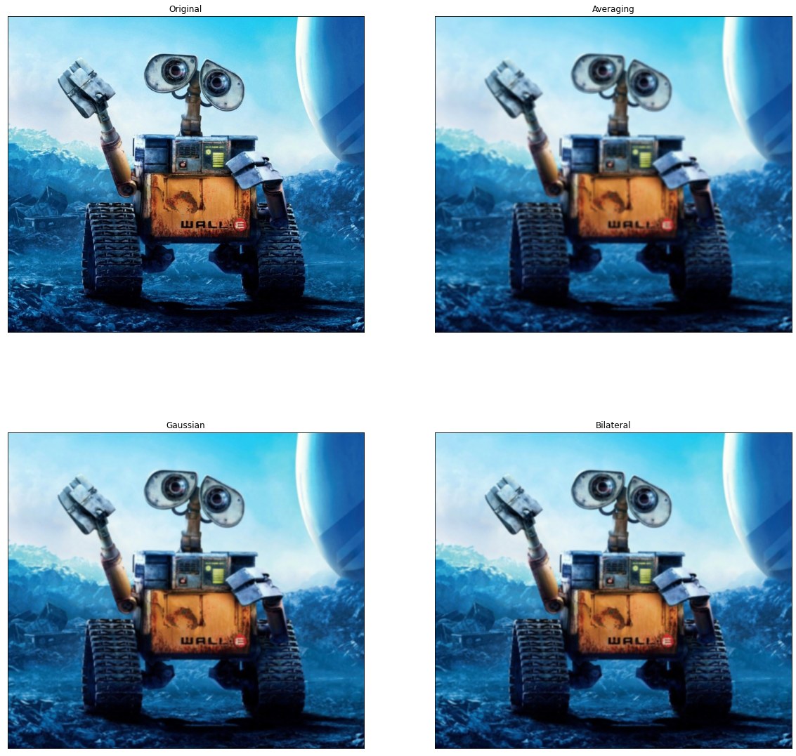
可以参考OpenCV图像处理基础变换和去噪了解更多 OpenCV 图像处理操作。
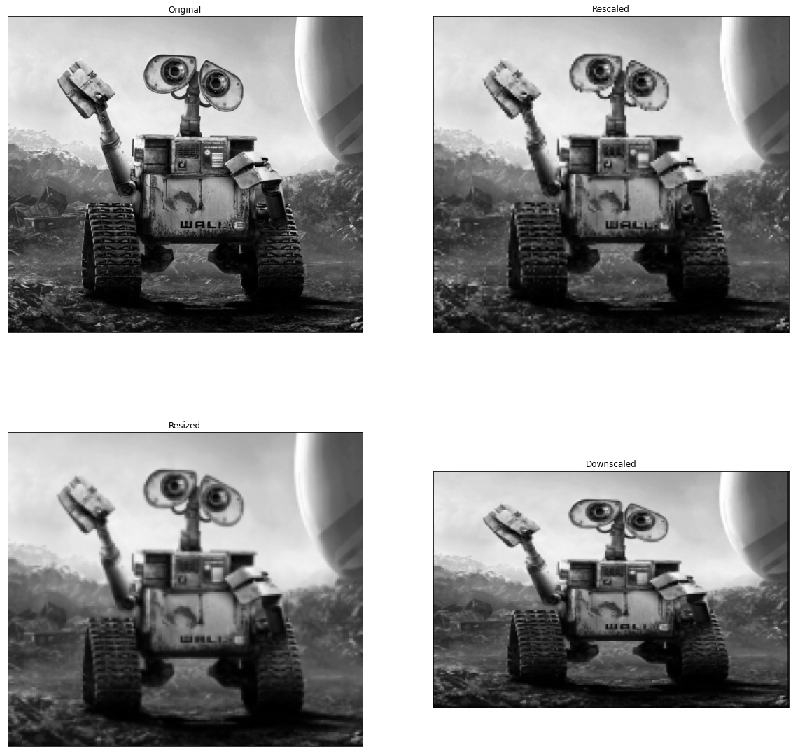
3、 Scikit-image
scikit-image是基于scipy的图像处理库它将图片作为numpy数组进行处理。
例如可以利用scikit-image改变图片比例scikit-image提供了rescale、resize以及downscale_local_mean等函数。
from skimage import data, color, io
from skimage.transform import rescale, resize, downscale_local_mean

image = color.rgb2gray(io.imread('h89817032p0.png'))

image_rescaled = rescale(image, 0.25, anti_aliasing=False)
image_resized = resize(image, (image.shape[0] // 4, image.shape[1] // 4),
                       anti_aliasing=True)
image_downscaled = downscale_local_mean(image, (4, 3))
plt.figure(figsize=(20,20))
plt.subplot(221),plt.imshow(image, cmap='gray'),plt.title('Original')
plt.xticks([]), plt.yticks([])
plt.subplot(222),plt.imshow(image_rescaled, cmap='gray'),plt.title('Rescaled')
plt.xticks([]), plt.yticks([])
plt.subplot(223),plt.imshow(image_resized, cmap='gray'),plt.title('Resized')
plt.xticks([]), plt.yticks([])
plt.subplot(224),plt.imshow(image_downscaled, cmap='gray'),plt.title('Downscaled')
plt.xticks([]), plt.yticks([])
plt.show()
4、 Python Imaging Library(PIL)
Python Imaging Library(PIL) 已经成为 Python 事实上的图像处理标准库了这是由于PIL 功能非常强大但API却非常简单易用。
但是由于PIL仅支持到 Python 2.7再加上年久失修于是一群志愿者在 PIL 的基础上创建了兼容的版本名字叫 Pillow支持最新 Python 3.x又加入了许多新特性因此我们可以跳过 PIL直接安装使用 Pillow。
5、 Pillow
使用 Pillow 生成字母验证码图片
from PIL import Image, ImageDraw, ImageFont, ImageFilter

import random

# 随机字母:
def rndChar():
    return chr(random.randint(65, 90))

# 随机颜色1:
def rndColor():
    return (random.randint(64, 255), random.randint(64, 255), random.randint(64, 255))

# 随机颜色2:
def rndColor2():
    return (random.randint(32, 127), random.randint(32, 127), random.randint(32, 127))

# 240 x 60:
width = 60 * 6
height = 60 * 6
image = Image.new('RGB', (width, height), (255, 255, 255))
# 创建Font对象:
font = ImageFont.truetype('/usr/share/fonts/wps-office/simhei.ttf', 60)
# 创建Draw对象:
draw = ImageDraw.Draw(image)
# 填充每个像素:
for x in range(width):
    for y in range(height):
        draw.point((x, y), fill=rndColor())
# 输出文字:
for t in range(6):
    draw.text((60 * t + 10, 150), rndChar(), font=font, fill=rndColor2())
# 模糊:
image = image.filter(ImageFilter.BLUR)
image.save('code.jpg', 'jpeg')

6、 SimpleCV
SimpleCV 是一个用于构建计算机视觉应用程序的开源框架。使用它可以访问高性能的计算机视觉库如 OpenCV而不必首先了解位深度、文件格式、颜色空间、缓冲区管理、特征值或矩阵等术语。但其对于 Python3 的支持很差很差在 Python3.7 中使用如下代码
from SimpleCV import Image, Color, Display
# load an image from imgur
img = Image('http://i.imgur.com/lfAeZ4n.png')
# use a keypoint detector to find areas of interest
feats = img.findKeypoints()
# draw the list of keypoints
feats.draw(color=Color.RED)
# show the  resulting image.
img.show()
# apply the stuff we found to the image.
output = img.applyLayers()
# save the results.
output.save('juniperfeats.png')
会报如下错误因此不建议在 Python3 中使用
SyntaxError: Missing parentheses in call to 'print'. Did you mean print('unit test')?
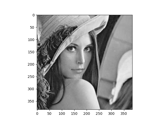
7、 Mahotas
Mahotas 是一个快速计算机视觉算法库其构建在 Numpy 之上目前拥有超过100种图像处理和计算机视觉功能并在不断增长。
使用 Mahotas 加载图像并对像素进行操作
import numpy as np
import mahotas
import mahotas.demos

from mahotas.thresholding import soft_threshold
from matplotlib import pyplot as plt
from os import path
f = mahotas.demos.load('lena', as_grey=True)
f = f[128:,128:]
plt.gray()
# Show the data:
print("Fraction of zeros in original image: {0}".format(np.mean(f==0)))
plt.imshow(f)
plt.show()
8、 Ilastik
Ilastik 能够给用户提供良好的基于机器学习的生物信息图像分析服务利用机器学习算法轻松地分割分类跟踪和计数细胞或其他实验数据。大多数操作都是交互式的并不需要机器学习专业知识。可以参考https://www.ilastik.org/documentation/basics/installation.html进行安装使用。
9、 Scikit-learn
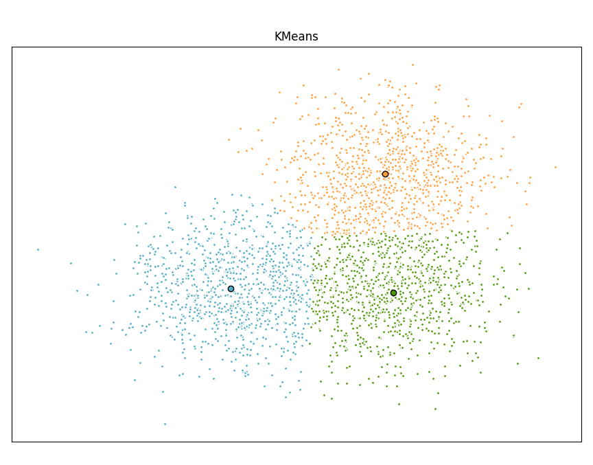
Scikit-learn 是针对 Python 编程语言的免费软件机器学习库。它具有各种分类回归和聚类算法包括支持向量机随机森林梯度提升k均值和 DBSCAN 等多种机器学习算法。
使用Scikit-learn实现KMeans算法
import time

import numpy as np
import matplotlib.pyplot as plt

from sklearn.cluster import MiniBatchKMeans, KMeans
from sklearn.metrics.pairwise import pairwise_distances_argmin
from sklearn.datasets import make_blobs

# Generate sample data
np.random.seed(0)

batch_size = 45
centers = [[1, 1], [-1, -1], [1, -1]]
n_clusters = len(centers)
X, labels_true = make_blobs(n_samples=3000, centers=centers, cluster_std=0.7)

# Compute clustering with Means

k_means = KMeans(init='k-means++', n_clusters=3, n_init=10)
t0 = time.time()
k_means.fit(X)
t_batch = time.time() - t0

# Compute clustering with MiniBatchKMeans

mbk = MiniBatchKMeans(init='k-means++', n_clusters=3, batch_size=batch_size,
                      n_init=10, max_no_improvement=10, verbose=0)
t0 = time.time()
mbk.fit(X)
t_mini_batch = time.time() - t0

# Plot result
fig = plt.figure(figsize=(8, 3))
fig.subplots_adjust(left=0.02, right=0.98, bottom=0.05, top=0.9)
colors = ['#4EACC5', '#FF9C34', '#4E9A06']

# We want to have the same colors for the same cluster from the
# MiniBatchKMeans and the KMeans algorithm. Let's pair the cluster centers per
# closest one.
k_means_cluster_centers = k_means.cluster_centers_
order = pairwise_distances_argmin(k_means.cluster_centers_,
                                  mbk.cluster_centers_)
mbk_means_cluster_centers = mbk.cluster_centers_[order]

k_means_labels = pairwise_distances_argmin(X, k_means_cluster_centers)
mbk_means_labels = pairwise_distances_argmin(X, mbk_means_cluster_centers)

# KMeans
for k, col in zip(range(n_clusters), colors):
    my_members = k_means_labels == k
    cluster_center = k_means_cluster_centers[k]
    plt.plot(X[my_members, 0], X[my_members, 1], 'w',
            markerfacecolor=col, marker='.')
    plt.plot(cluster_center[0], cluster_center[1], 'o', markerfacecolor=col,
            markeredgecolor='k', markersize=6)
plt.title('KMeans')
plt.xticks(())
plt.yticks(())

plt.show()
10、 SciPy
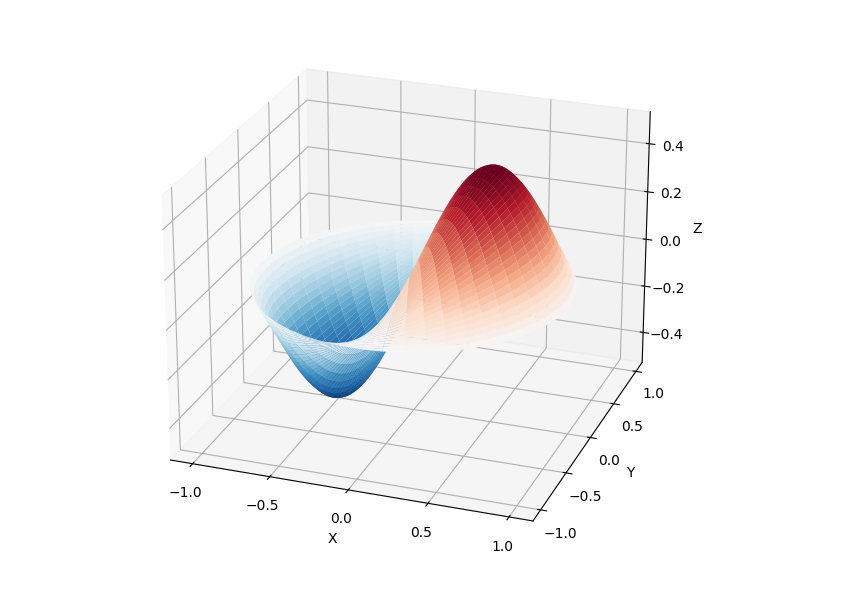
SciPy 库提供了许多用户友好和高效的数值计算如数值积分、插值、优化、线性代数等。
SciPy 库定义了许多数学物理的特殊函数包括椭圆函数、贝塞尔函数、伽马函数、贝塔函数、超几何函数、抛物线圆柱函数等等。
from scipy import special
import matplotlib.pyplot as plt
import numpy as np

def drumhead_height(n, k, distance, angle, t):
    kth_zero = special.jn_zeros(n, k)[-1]
    return np.cos(t) * np.cos(n*angle) * special.jn(n, distance*kth_zero)

theta = np.r_[0:2*np.pi:50j]
radius = np.r_[0:1:50j]
x = np.array([r * np.cos(theta) for r in radius])
y = np.array([r * np.sin(theta) for r in radius])
z = np.array([drumhead_height(1, 1, r, theta, 0.5) for r in radius])


fig = plt.figure()
ax = fig.add_axes(rect=(0, 0.05, 0.95, 0.95), projection='3d')
ax.plot_surface(x, y, z, rstride=1, cstride=1, cmap='RdBu_r', vmin=-0.5, vmax=0.5)
ax.set_xlabel('X')
ax.set_ylabel('Y')
ax.set_xticks(np.arange(-1, 1.1, 0.5))
ax.set_yticks(np.arange(-1, 1.1, 0.5))
ax.set_zlabel('Z')
plt.show()
11、 NLTK
NLTK 是构建Python程序以处理自然语言的库。它为50多个语料库和词汇资源(如 WordNet )提供了易于使用的接口以及一套用于分类、分词、词干、标记、解析和语义推理的文本处理库、工业级自然语言处理 (Natural Language Processing, NLP) 库的包装器。
NLTK被称为 “a wonderful tool for teaching, and working in, computational linguistics using Python”。
import nltk
from nltk.corpus import treebank

# 首次使用需要下载
nltk.download('punkt')
nltk.download('averaged_perceptron_tagger')
nltk.download('maxent_ne_chunker')
nltk.download('words')
nltk.download('treebank')

sentence = """At eight o'clock on Thursday morning Arthur didn't feel very good."""
# Tokenize
tokens = nltk.word_tokenize(sentence)
tagged = nltk.pos_tag(tokens)

# Identify named entities
entities = nltk.chunk.ne_chunk(tagged)

# Display a parse tree
t = treebank.parsed_sents('wsj_0001.mrg')[0]
t.draw()
12、 spaCy
spaCy 是一个免费的开源库用于 Python 中的高级 NLP。它可以用于构建处理大量文本的应用程序也可以用来构建信息提取或自然语言理解系统或者对文本进行预处理以进行深度学习。
  import spacy

  texts = [
      "Net income was $9.4 million compared to the prior year of $2.7 million.",
      "Revenue exceeded twelve billion dollars, with a loss of $1b.",
  ]

  nlp = spacy.load("en_core_web_sm")
  for doc in nlp.pipe(texts, disable=["tok2vec", "tagger", "parser", "attribute_ruler", "lemmatizer"]):
      # Do something with the doc here
      print([(ent.text, ent.label_) for ent in doc.ents])
nlp.pipe 生成 Doc 对象因此我们可以对它们进行迭代并访问命名实体预测
[('$9.4 million', 'MONEY'), ('the prior year', 'DATE'), ('$2.7 million', 'MONEY')]
[('twelve billion dollars', 'MONEY'), ('1b', 'MONEY')]
13、 LibROSA
librosa 是一个用于音乐和音频分析的 Python 库它提供了创建音乐信息检索系统所必需的功能和函数。
# Beat tracking example
import librosa

# 1. Get the file path to an included audio example
filename = librosa.example('nutcracker')

# 2. Load the audio as a waveform `y`
#    Store the sampling rate as `sr`
y, sr = librosa.load(filename)

# 3. Run the default beat tracker
tempo, beat_frames = librosa.beat.beat_track(y=y, sr=sr)
print('Estimated tempo: {:.2f} beats per minute'.format(tempo))

# 4. Convert the frame indices of beat events into timestamps
beat_times = librosa.frames_to_time(beat_frames, sr=sr)
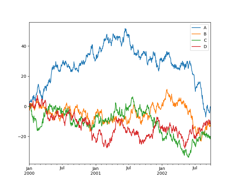
14、 Pandas
Pandas 是一个快速、强大、灵活且易于使用的开源数据分析和操作工具 Pandas 可以从各种文件格式比如 CSV、JSON、SQL、Microsoft Excel 导入数据可以对各种数据进行运算操作比如归并、再成形、选择还有数据清洗和数据加工特征。Pandas 广泛应用在学术、金融、统计学等各个数据分析领域。
import matplotlib.pyplot as plt
import pandas as pd
import numpy as np

ts = pd.Series(np.random.randn(1000), index=pd.date_range("1/1/2000", periods=1000))
ts = ts.cumsum()

df = pd.DataFrame(np.random.randn(1000, 4), index=ts.index, columns=list("ABCD"))
df = df.cumsum()
df.plot()
plt.show()
15、 Matplotlib
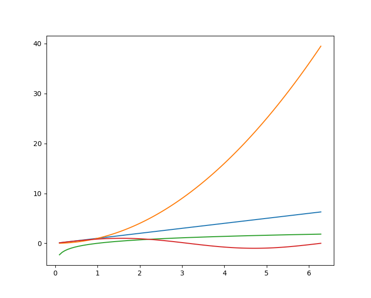
Matplotlib 是Python的绘图库它提供了一整套和 matlab 相似的命令 API可以生成出版质量级别的精美图形Matplotlib 使绘图变得非常简单在易用性和性能间取得了优异的平衡。
使用 Matplotlib 绘制多曲线图
# plot_multi_curve.py
import numpy as np
import matplotlib.pyplot as plt
x = np.linspace(0.1, 2 * np.pi, 100)
y_1 = x
y_2 = np.square(x)
y_3 = np.log(x)
y_4 = np.sin(x)
plt.plot(x,y_1)
plt.plot(x,y_2)
plt.plot(x,y_3)
plt.plot(x,y_4)
plt.show()
 有关更多
有关更多Matplotlib绘图的介绍可以参考此前博文———Python-Matplotlib可视化。
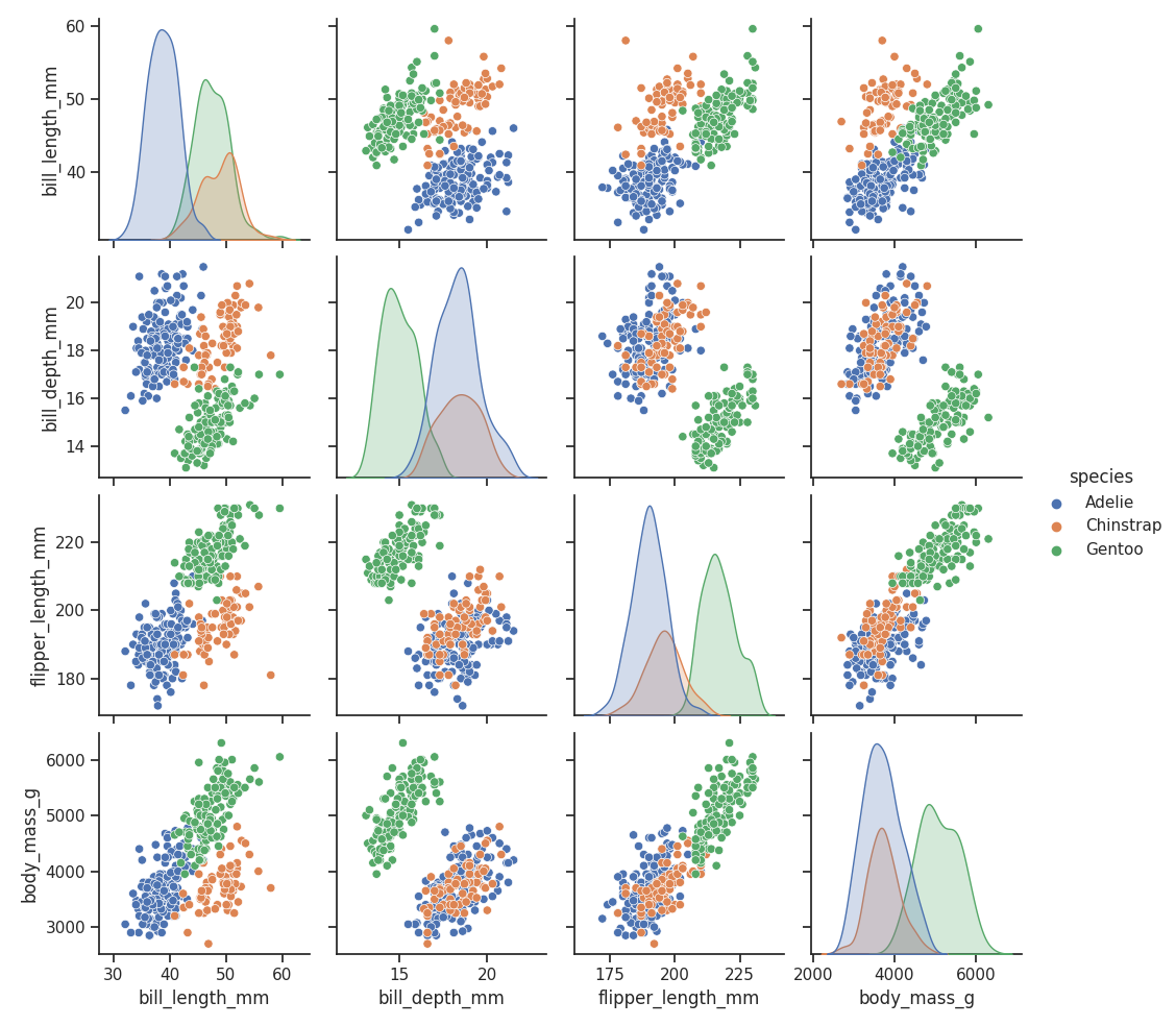
16、 Seaborn
Seaborn 是在 Matplotlib 的基础上进行了更高级的API封装的Python数据可视化库从而使得作图更加容易应该把 Seaborn 视为 Matplotlib 的补充而不是替代物。
import seaborn as sns
import matplotlib.pyplot as plt
sns.set_theme(style="ticks")

df = sns.load_dataset("penguins")
sns.pairplot(df, hue="species")
plt.show()
17、 Orange
Orange 是一个开源的数据挖掘和机器学习软件提供了一系列的数据探索、可视化、预处理以及建模组件。Orange 拥有漂亮直观的交互式用户界面非常适合新手进行探索性数据分析和可视化展示同时高级用户也可以将其作为 Python 的一个编程模块进行数据操作和组件开发。
使用 pip 即可安装 Orange好评~
$ pip install orange3
安装完成后在命令行输入 orange-canvas 命令即可启动 Orange 图形界面
$ orange-canvas
启动完成后即可看到 Orange 图形界面进行各种操作。

18、 PyBrain
PyBrain 是 Python 的模块化机器学习库。它的目标是为机器学习任务和各种预定义的环境提供灵活、易于使用且强大的算法来测试和比较算法。PyBrain 是 Python-Based Reinforcement Learning, Artificial Intelligence and Neural Network Library 的缩写。
我们将利用一个简单的例子来展示 PyBrain 的用法构建一个多层感知器 (Multi Layer Perceptron, MLP)。
首先我们创建一个新的前馈网络对象
from pybrain.structure import FeedForwardNetwork

n = FeedForwardNetwork()
接下来构建输入、隐藏和输出层
from pybrain.structure import LinearLayer, SigmoidLayer

inLayer = LinearLayer(2)
hiddenLayer = SigmoidLayer(3)
outLayer = LinearLayer(1)
为了使用所构建的层必须将它们添加到网络中
n.addInputModule(inLayer)
n.addModule(hiddenLayer)
n.addOutputModule(outLayer)
可以添加多个输入和输出模块。为了向前计算和反向误差传播网络必须知道哪些层是输入、哪些层是输出。
这就需要明确确定它们应该如何连接。为此我们使用最常见的连接类型全连接层由 FullConnection 类实现
from pybrain.structure import FullConnection
in_to_hidden = FullConnection(inLayer, hiddenLayer)
hidden_to_out = FullConnection(hiddenLayer, outLayer)
与层一样我们必须明确地将它们添加到网络中
n.addConnection(in_to_hidden)
n.addConnection(hidden_to_out)
所有元素现在都已准备就位最后我们需要调用.sortModules()方法使MLP可用
n.sortModules()
这个调用会执行一些内部初始化这在使用网络之前是必要的。
19、 Milk
MILK(MACHINE LEARNING TOOLKIT) 是 Python 语言的机器学习工具包。它主要是包含许多分类器比如 SVMS、K-NN、随机森林以及决策树中使用监督分类法它还可执行特征选择可以形成不同的例如无监督学习、密切关系传播和由 MILK 支持的 K-means 聚类等分类系统。
使用 MILK 训练一个分类器
import numpy as np
import milk
features = np.random.rand(100,10)
labels = np.zeros(100)
features[50:] += .5
labels[50:] = 1
learner = milk.defaultclassifier()
model = learner.train(features, labels)

# Now you can use the model on new examples:
example = np.random.rand(10)
print(model.apply(example))
example2 = np.random.rand(10)
example2 += .5
print(model.apply(example2))
20、 TensorFlow
TensorFlow 是一个端到端开源机器学习平台。它拥有一个全面而灵活的生态系统一般可以将其分为 TensorFlow1.x 和 TensorFlow2.xTensorFlow1.x 与 TensorFlow2.x 的主要区别在于 TF1.x 使用静态图而 TF2.x 使用Eager Mode动态图。
这里主要使用TensorFlow2.x作为示例展示在 TensorFlow2.x 中构建卷积神经网络 (Convolutional Neural Network, CNN)。
import tensorflow as tf

from tensorflow.keras import datasets, layers, models

# 数据加载
(train_images, train_labels), (test_images, test_labels) = datasets.cifar10.load_data()

# 数据预处理
train_images, test_images = train_images / 255.0, test_images / 255.0

# 模型构建
model = models.Sequential()
model.add(layers.Conv2D(32, (3, 3), activation='relu', input_shape=(32, 32, 3)))
model.add(layers.MaxPooling2D((2, 2)))
model.add(layers.Conv2D(64, (3, 3), activation='relu'))
model.add(layers.MaxPooling2D((2, 2)))
model.add(layers.Conv2D(64, (3, 3), activation='relu'))
model.add(layers.Flatten())
model.add(layers.Dense(64, activation='relu'))
model.add(layers.Dense(10))

# 模型编译与训练
model.compile(optimizer='adam',
              loss=tf.keras.losses.SparseCategoricalCrossentropy(from_logits=True),
              metrics=['accuracy'])
history = model.fit(train_images, train_labels, epochs=10,
                    validation_data=(test_images, test_labels))
想要了解更多Tensorflow2.x的示例可以参考专栏 Tensorflow.
21、 PyTorch
PyTorch 的前身是 Torch其底层和 Torch 框架一样但是使用 Python 重新写了很多内容不仅更加灵活支持动态图而且提供了 Python 接口。
# 导入库
import torch
from torch import nn
from torch.utils.data import DataLoader
from torchvision import datasets
from torchvision.transforms import ToTensor, Lambda, Compose
import matplotlib.pyplot as plt

# 模型构建
device = "cuda" if torch.cuda.is_available() else "cpu"
print("Using {} device".format(device))

# Define model
class NeuralNetwork(nn.Module):
    def __init__(self):
        super(NeuralNetwork, self).__init__()
        self.flatten = nn.Flatten()
        self.linear_relu_stack = nn.Sequential(
            nn.Linear(28*28, 512),
            nn.ReLU(),
            nn.Linear(512, 512),
            nn.ReLU(),
            nn.Linear(512, 10),
            nn.ReLU()
        )

    def forward(self, x):
        x = self.flatten(x)
        logits = self.linear_relu_stack(x)
        return logits

model = NeuralNetwork().to(device)

# 损失函数和优化器
loss_fn = nn.CrossEntropyLoss()
optimizer = torch.optim.SGD(model.parameters(), lr=1e-3)

# 模型训练
def train(dataloader, model, loss_fn, optimizer):
    size = len(dataloader.dataset)
    for batch, (X, y) in enumerate(dataloader):
        X, y = X.to(device), y.to(device)

        # Compute prediction error
        pred = model(X)
        loss = loss_fn(pred, y)

        # Backpropagation
        optimizer.zero_grad()
        loss.backward()
        optimizer.step()

        if batch % 100 == 0:
            loss, current = loss.item(), batch * len(X)
            print(f"loss: {loss:>7f}  [{current:>5d}/{size:>5d}]")
22、 Theano
Theano 是一个 Python 库它允许定义、优化和有效地计算涉及多维数组的数学表达式建在 NumPy 之上。
在 Theano 中实现计算雅可比矩阵
import theano
import theano.tensor as T
x = T.dvector('x')
y = x ** 2
J, updates = theano.scan(lambda i, y,x : T.grad(y[i], x), sequences=T.arange(y.shape[0]), non_sequences=[y,x])
f = theano.function([x], J, updates=updates)
f([4, 4])
23、 Keras
Keras 是一个用 Python 编写的高级神经网络 API它能够以 TensorFlow, CNTK, 或者 Theano 作为后端运行。Keras 的开发重点是支持快速的实验能够以最小的时延把想法转换为实验结果。
from keras.models import Sequential
from keras.layers import Dense

# 模型构建
model = Sequential()
model.add(Dense(units=64, activation='relu', input_dim=100))
model.add(Dense(units=10, activation='softmax'))

# 模型编译与训练
model.compile(loss='categorical_crossentropy',
              optimizer='sgd',
              metrics=['accuracy'])
model.fit(x_train, y_train, epochs=5, batch_size=32)
24、 Caffe
在 Caffe2 官方网站上这样说道Caffe2 现在是 PyTorch 的一部分。虽然这些 api 将继续工作但鼓励使用 PyTorch api。
25、 MXNet
MXNet 是一款设计为效率和灵活性的深度学习框架。它允许混合符号编程和命令式编程从而最大限度提高效率和生产力。
使用 MXNet 构建手写数字识别模型
import mxnet as mx
from mxnet import gluon
from mxnet.gluon import nn
from mxnet import autograd as ag
import mxnet.ndarray as F

# 数据加载
mnist = mx.test_utils.get_mnist()
batch_size = 100
train_data = mx.io.NDArrayIter(mnist['train_data'], mnist['train_label'], batch_size, shuffle=True)
val_data = mx.io.NDArrayIter(mnist['test_data'], mnist['test_label'], batch_size)

# CNN模型
class Net(gluon.Block):
    def __init__(self, **kwargs):
        super(Net, self).__init__(**kwargs)
        self.conv1 = nn.Conv2D(20, kernel_size=(5,5))
        self.pool1 = nn.MaxPool2D(pool_size=(2,2), strides = (2,2))
        self.conv2 = nn.Conv2D(50, kernel_size=(5,5))
        self.pool2 = nn.MaxPool2D(pool_size=(2,2), strides = (2,2))
        self.fc1 = nn.Dense(500)
        self.fc2 = nn.Dense(10)

    def forward(self, x):
        x = self.pool1(F.tanh(self.conv1(x)))
        x = self.pool2(F.tanh(self.conv2(x)))
        # 0 means copy over size from corresponding dimension.
        # -1 means infer size from the rest of dimensions.
        x = x.reshape((0, -1))
        x = F.tanh(self.fc1(x))
        x = F.tanh(self.fc2(x))
        return x
net = Net()
# 初始化与优化器定义
# set the context on GPU is available otherwise CPU
ctx = [mx.gpu() if mx.test_utils.list_gpus() else mx.cpu()]
net.initialize(mx.init.Xavier(magnitude=2.24), ctx=ctx)
trainer = gluon.Trainer(net.collect_params(), 'sgd', {'learning_rate': 0.03})

# 模型训练
# Use Accuracy as the evaluation metric.
metric = mx.metric.Accuracy()
softmax_cross_entropy_loss = gluon.loss.SoftmaxCrossEntropyLoss()

for i in range(epoch):
    # Reset the train data iterator.
    train_data.reset()
    for batch in train_data:
        data = gluon.utils.split_and_load(batch.data[0], ctx_list=ctx, batch_axis=0)
        label = gluon.utils.split_and_load(batch.label[0], ctx_list=ctx, batch_axis=0)
        outputs = []
        # Inside training scope
        with ag.record():
            for x, y in zip(data, label):
                z = net(x)
                # Computes softmax cross entropy loss.
                loss = softmax_cross_entropy_loss(z, y)
                # Backpropogate the error for one iteration.
                loss.backward()
                outputs.append(z)
        metric.update(label, outputs)
        trainer.step(batch.data[0].shape[0])
    # Gets the evaluation result.
    name, acc = metric.get()
    # Reset evaluation result to initial state.
    metric.reset()
    print('training acc at epoch %d: %s=%f'%(i, name, acc))
26、 PaddlePaddle
飞桨 (PaddlePaddle) 以百度多年的深度学习技术研究和业务应用为基础集深度学习核心训练和推理框架、基础模型库、端到端开发套件、丰富的工具组件于一体。是中国首个自主研发、功能完备、开源开放的产业级深度学习平台。
使用 PaddlePaddle 实现 LeNtet5
# 导入需要的包
import paddle
import numpy as np
from paddle.nn import Conv2D, MaxPool2D, Linear

## 组网
import paddle.nn.functional as F

# 定义 LeNet 网络结构
class LeNet(paddle.nn.Layer):
    def __init__(self, num_classes=1):
        super(LeNet, self).__init__()
        # 创建卷积和池化层
        # 创建第1个卷积层
        self.conv1 = Conv2D(in_channels=1, out_channels=6, kernel_size=5)
        self.max_pool1 = MaxPool2D(kernel_size=2, stride=2)
        # 尺寸的逻辑池化层未改变通道数当前通道数为6
        # 创建第2个卷积层
        self.conv2 = Conv2D(in_channels=6, out_channels=16, kernel_size=5)
        self.max_pool2 = MaxPool2D(kernel_size=2, stride=2)
        # 创建第3个卷积层
        self.conv3 = Conv2D(in_channels=16, out_channels=120, kernel_size=4)
        # 尺寸的逻辑输入层将数据拉平[B,C,H,W] -> [B,C*H*W]
        # 输入size是[28,28]经过三次卷积和两次池化之后C*H*W等于120
        self.fc1 = Linear(in_features=120, out_features=64)
        # 创建全连接层第一个全连接层的输出神经元个数为64 第二个全连接层输出神经元个数为分类标签的类别数
        self.fc2 = Linear(in_features=64, out_features=num_classes)
    # 网络的前向计算过程
    def forward(self, x):
        x = self.conv1(x)
        # 每个卷积层使用Sigmoid激活函数后面跟着一个2x2的池化
        x = F.sigmoid(x)
        x = self.max_pool1(x)
        x = F.sigmoid(x)
        x = self.conv2(x)
        x = self.max_pool2(x)
        x = self.conv3(x)
        # 尺寸的逻辑输入层将数据拉平[B,C,H,W] -> [B,C*H*W]
        x = paddle.reshape(x, [x.shape[0], -1])
        x = self.fc1(x)
        x = F.sigmoid(x)
        x = self.fc2(x)
        return x
27、 CNTK
CNTK(Cognitive Toolkit) 是一个深度学习工具包通过有向图将神经网络描述为一系列计算步骤。在这个有向图中叶节点表示输入值或网络参数而其他节点表示对其输入的矩阵运算。CNTK 可以轻松地实现和组合流行的模型类型如 CNN 等。
CNTK 用网络描述语言 (network description language, NDL) 描述一个神经网络。 简单的说要描述输入的 feature输入的 label一些参数参数和输入之间的计算关系以及目标节点是什么。
NDLNetworkBuilder=[

    run=ndlLR

    ndlLR=[
      # sample and label dimensions
      SDim=$dimension$
      LDim=1

      features=Input(SDim, 1)
      labels=Input(LDim, 1)

      # parameters to learn
      B0 = Parameter(4)
      W0 = Parameter(4, SDim)


      B = Parameter(LDim)
      W = Parameter(LDim, 4)

      # operations
      t0 = Times(W0, features)
      z0 = Plus(t0, B0)
      s0 = Sigmoid(z0)

      t = Times(W, s0)
      z = Plus(t, B)
      s = Sigmoid(z)

      LR = Logistic(labels, s)
      EP = SquareError(labels, s)

      # root nodes
      FeatureNodes=(features)
      LabelNodes=(labels)
      CriteriaNodes=(LR)
      EvalNodes=(EP)
      OutputNodes=(s,t,z,s0,W0)
    ]
  ]
总结与分类
python 常用机器学习及深度学习库总结
| 库名 | 官方网站 | 简介 |
|---|---|---|
| NumPy | http://www.numpy.org/ | 提供对大型多维阵列的支持NumPy是计算机视觉中的一个关键库因为图像可以表示为多维数组将图像表示为NumPy数组有许多优点 |
| OpenCV | https://opencv.org/ | 开源的计算机视觉库 |
| Scikit-image | https:// scikit-image.org/ | 图像处理算法的集合,由scikit-image操作的图像只能是NumPy数组 |
| Python Imaging Library(PIL) | http://www.pythonware.com/products/pil/ | 图像处理库提供强大的图像处理和图形功能 |
| Pillow | https://pillow.readthedocs.io/ | PIL的一个分支 |
| SimpleCV | http://simplecv.org/ | 计算机视觉框架提供了处理图像处理的关键功能 |
| Mahotas | https://mahotas.readthedocs.io/ | 提供了用于图像处理和计算机视觉的一组函数它最初是为生物图像信息学而设计的但是现在它在其他领域也发挥了重要作用它完全基于numpy数组作为其数据类型 |
| Ilastik | http://ilastik.org/ | 用户友好且简单的交互式图像分割、分类和分析工具 |
| Scikit-learn | http://scikit-learn.org/ | 机器学习库具有各种分类、回归和聚类算法 |
| SciPy | https://www.scipy.org/ | 科学和技术计算库 |
| NLTK | https://www.nltk.org/ | 处理自然语言数据的库和程序 |
| spaCy | https://spacy.io/ | 开源软件库用于Python中的高级自然语言处理 |
| LibROSA | https://librosa.github.io/librosa/ | 用于音乐和音频处理的库 |
| Pandas | https://pandas.pydata.org/ | 构建在NumPy之上的库提供高级数据计算工具和易于使用的数据结构 |
| Matplotlib | https://matplotlib.org | 绘图库它提供了一整套和 matlab 相似的命令 API可以生成所需的出版质量级别的图形 |
| Seaborn | https://seaborn.pydata.org/ | 是建立在Matplotlib之上的绘图库 |
| Orange | https://orange.biolab.si/ | 面向新手和专家的开源机器学习和数据可视化工具包 |
| PyBrain | http://pybrain.org/ | 机器学习库为机器学习提供易于使用的最新算法 |
| Milk | http://luispedro.org/software/milk/ | 机器学习工具箱主要用于监督学习中的多分类问题 |
| TensorFlow | https://www.tensorflow.org/ | 开源的机器学习和深度学习库 |
| PyTorch | https://pytorch.org/ | 开源的机器学习和深度学习库 |
| Theano | http://deeplearning.net/software/theano/ | 用于快速数学表达式、求值和计算的库已编译为可在CPU和GPU架构上运行 |
| Keras | https://keras.io/ | 高级深度学习库可以在 TensorFlow、CNTK、Theano 或 Microsoft Cognitive Toolkit 之上运行 |
| Caffe2 | https://caffe2.ai/ | Caffe2 是一个兼具表现力、速度和模块性的深度学习框架是 Caffe 的实验性重构能以更灵活的方式组织计算 |
| MXNet | https://mxnet.apache.org/ | 设计为效率和灵活性的深度学习框架允许混合符号编程和命令式编程 |
| PaddlePaddle | https://www.paddlepaddle.org.cn | 以百度多年的深度学习技术研究和业务应用为基础集深度学习核心训练和推理框架、基础模型库、端到端开发套件、丰富的工具组件于一体 |
| CNTK | https://cntk.ai/ | 深度学习工具包通过有向图将神经网络描述为一系列计算步骤。在这个有向图中叶节点表示输入值或网络参数而其他节点表示对其输入的矩阵运算 |
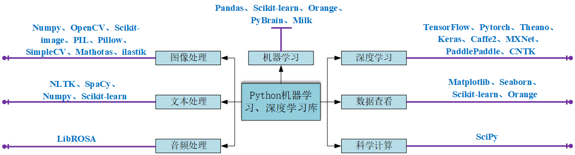
分类
可以根据其主要用途将这些库进行分类
| 类别 | 库 |
|---|---|
| 图像处理 | NumPy、OpenCV、scikit image、PIL、Pillow、SimpleCV、Mahotas、ilastik |
| 文本处理 | NLTK、spaCy、NumPy、scikit learn、PyTorch |
| 音频处理 | LibROSA |
| 机器学习 | pandas, scikit-learn, Orange, PyBrain, Milk |
| 数据查看 | Matplotlib、Seaborn、scikit-learn、Orange |
| 深度学习 | TensorFlow、Pytorch、Theano、Keras、Caffe2、MXNet、PaddlePaddle、CNTK |
| 科学计算 | SciPy |
更多
有关 AI 和机器学习的其他 Python 库和包可以访问https://python.libhunt.com/packages/artificial-intelligence.