【机器学习】逻辑回归(实战)
| 阿里云国内75折 回扣 微信号:monov8 |
| 阿里云国际,腾讯云国际,低至75折。AWS 93折 免费开户实名账号 代冲值 优惠多多 微信号:monov8 飞机:@monov6 |
逻辑回归实战
目录
实战部分将结合着 理论部分 进行旨在帮助理解和强化实操以下代码将基于 jupyter notebook 进行。
一、准备工作设置 jupyter notebook 中的字体大小样式等
import numpy as np
import os
%matplotlib inline
import matplotlib
import matplotlib.pyplot as plt
plt.rcParams['axes.labelsize'] = 14
plt.rcParams['xtick.labelsize'] = 12
plt.rcParams['ytick.labelsize'] = 12
import warnings
warnings.filterwarnings('ignore')
np. random.seed(42)
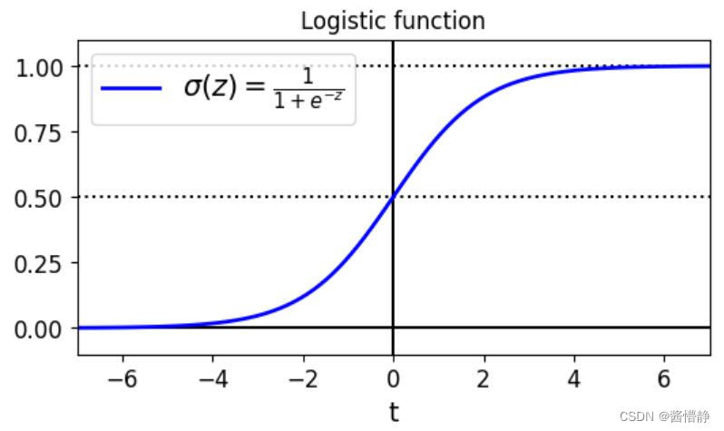
二、绘制 sigmoid 函数: σ ( z ) = 1 1 + e − z \sigma(z)=\frac{1}{1+e^{-z}} σ(z)=1+e−z1
AbsoluteLimiteLength = 7
t = np.linspace(-AbsoluteLimiteLength,AbsoluteLimiteLength,100)
sig = 1/ (1 + np.exp(-t))
plt.figure(figsize=(6,4))
plt.plot([-AbsoluteLimiteLength,AbsoluteLimiteLength], [0,0], "k-")
plt.plot([-AbsoluteLimiteLength,AbsoluteLimiteLength], [0.5,0.5], "k:")
plt.plot([-AbsoluteLimiteLength,AbsoluteLimiteLength], [1,1], "k:")
plt.plot([0,0],[-1.1, 1.1], "k-")
plt.plot(t, sig, "b-", linewidth=2, label= r"$\sigma(z) = \frac{1} {1 + e^{-z}}$")
plt.xlabel("t")
plt.legend(loc="upper left", fontsize=15)
plt.axis([-AbsoluteLimiteLength, AbsoluteLimiteLength, -0.1, 1.1])
plt.title('Logistic function')
plt.show ()
绘制出构建的数据散点图
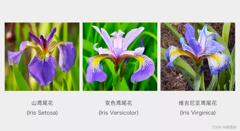
三、查看鸢尾花数据集
鸢尾花数据集:含有 3 个类别每个类别有 50 条数据所有数据均有 4 个特征分布是:萼片长度、萼片宽度、花瓣长度、花瓣宽度。
1、加载 iris 数据集并查看
# 加载 iris 数据集
from sklearn import datasets
iris = datasets.load_iris()

# 下面的命令可以查看 iris 数据集有哪些 keys 值是可以调用的
list(iris.keys())
Out
	['data',
	 'target',
	 'frame',
	 'target_names',
	 'DESCR',
	 'feature_names',
	 'filename',
	 'data_module']
# 打印数据的信息
print(iris.DESCR)
	.. _iris_dataset:

	Iris plants dataset
	--------------------

	**Data Set Characteristics:**

	    :Number of Instances: 150 (50 in each of three classes)
	    :Number of Attributes: 4 numeric, predictive attributes and the class
	    :Attribute Information:
	        - sepal length in cm
	        - sepal width in cm
	        - petal length in cm
	        - petal width in cm
	        - class:
	                - Iris-Setosa
	                - Iris-Versicolour
	                - Iris-Virginica

	    :Summary Statistics:

	    ============== ==== ==== ======= ===== ====================
	                    Min  Max   Mean    SD   Class Correlation
	    ============== ==== ==== ======= ===== ====================
	    sepal length:   4.3  7.9   5.84   0.83    0.7826
	    sepal width:    2.0  4.4   3.05   0.43   -0.4194
	    petal length:   1.0  6.9   3.76   1.76    0.9490  (high!)
	    petal width:    0.1  2.5   1.20   0.76    0.9565  (high!)
	    ============== ==== ==== ======= ===== ====================

	    :Missing Attribute Values: None
	    :Class Distribution: 33.3% for each of 3 classes.
	    :Creator: R.A. Fisher
	    :Donor: Michael Marshall (MARSHALL%PLU@io.arc.nasa.gov)
	    :Date: July, 1988

	The famous Iris database, first used by Sir R.A. Fisher. The dataset is taken
	from Fisher's paper. Note that it's the same as in R, but not as in the UCI
	Machine Learning Repository, which has two wrong data points.

	This is perhaps the best known database to be found in the
	pattern recognition literature.  Fisher's paper is a classic in the field and
	is referenced frequently to this day.  (See Duda & Hart, for example.)  The
	data set contains 3 classes of 50 instances each, where each class refers to a
	type of iris plant.  One class is linearly separable from the other 2; the
	latter are NOT linearly separable from each other.

	.. topic:: References

	   - Fisher, R.A. "The use of multiple measurements in taxonomic problems"
	     Annual Eugenics, 7, Part II, 179-188 (1936); also in "Contributions to
	     Mathematical Statistics" (John Wiley, NY, 1950).
	   - Duda, R.O., & Hart, P.E. (1973) Pattern Classification and Scene Analysis.
	     (Q327.D83) John Wiley & Sons.  ISBN 0-471-22361-1.  See page 218.
	   - Dasarathy, B.V. (1980) "Nosing Around the Neighborhood: A New System
	     Structure and Classification Rule for Recognition in Partially Exposed
	     Environments".  IEEE Transactions on Pattern Analysis and Machine
	     Intelligence, Vol. PAMI-2, No. 1, 67-71.
	   - Gates, G.W. (1972) "The Reduced Nearest Neighbor Rule".  IEEE Transactions
	     on Information Theory, May 1972, 431-433.
	   - See also: 1988 MLC Proceedings, 54-64.  Cheeseman et al"s AUTOCLASS II
	     conceptual clustering system finds 3 classes in the data.
	   - Many, many more ...
2、设计二分类实验
选取其中 Virginica 类型在数据集中为第 3 类index = 2的鸢尾花作为一类、剩余的鸢尾花作为另一类。
注:为了便于读者在后面绘制决策边界时更容易理解接下来的回归实验仅选取鸢尾花数据集中的一个特征来进行。
# 这里选择 iris 数据集的第 3 个特征作为回归实验的 X 数组
X = iris['data'][:,3:]
print("查看训练数据的前 10 项:")
print(X[:10])
print()

# 将 Virginica 花的标签设置为 1其余为 0
y = (iris['target'] == 2).astype(np.int)
print("查看数据对应的标签:")
print(y)
Out
	查看训练数据的前 10 项:
	[[0.2]
	 [0.2]
	 [0.2]
	 [0.2]
	 [0.2]
	 [0.4]
	 [0.3]
	 [0.2]
	 [0.2]
	 [0.1]]

	查看数据对应的标签:
	[0 0 0 0 0 0 0 0 0 0 0 0 0 0 0 0 0 0 0 0 0 0 0 0 0 0 0 0 0 0 0 0 0 0 0 0 0
	 0 0 0 0 0 0 0 0 0 0 0 0 0 0 0 0 0 0 0 0 0 0 0 0 0 0 0 0 0 0 0 0 0 0 0 0 0
	 0 0 0 0 0 0 0 0 0 0 0 0 0 0 0 0 0 0 0 0 0 0 0 0 0 0 1 1 1 1 1 1 1 1 1 1 1
	 1 1 1 1 1 1 1 1 1 1 1 1 1 1 1 1 1 1 1 1 1 1 1 1 1 1 1 1 1 1 1 1 1 1 1 1 1
	 1 1]
四、实验:逻辑回归
1、分类器的构建
# 导入包
from sklearn.linear_model import LogisticRegression
log_res = LogisticRegression()

# 训练分类器
log_res.fit(X,y)
# 构建测试数据只有一个特征
# reshape(-1,1)表示将指定数据的全部内容“-1”置为一个 1 维的的数组“1”
X_new = np.linspace(0,3,1000).reshape(-1,1)

# 查看构建数据的前 10 项
print(X_new[:10])
Out
	[[0.        ]
	 [0.003003  ]
	 [0.00600601]
	 [0.00900901]
	 [0.01201201]
	 [0.01501502]
	 [0.01801802]
	 [0.02102102]
	 [0.02402402]
	 [0.02702703]]
# 得到预测结果为了便于进行可视化展示这里的预测结果不返回 0 与 1 的二值结果而是得到一组概率值
# CLF.predict()函数默认将所有的概率按 0.5 作为阈值来划分出二值结果
# CLF.predict_proba()函数则是返回所有数据的概率值其返回类型是一个 [][2] 的数组第一个维度为“预测目标为 1 的概率”第二个维度为“预测目标为 0 的概率”
y_proba = log_res.predict_proba(X_new)
print(np.shape(y_proba))
print(y_proba[:10])
Out
	(1000, 2)
	[[9.99250016e-01 7.49984089e-04]
	 [9.99240201e-01 7.59799387e-04]
	 [9.99230257e-01 7.69743043e-04]
	 [9.99220183e-01 7.79816732e-04]
	 [9.99209978e-01 7.90022153e-04]
	 [9.99199639e-01 8.00361024e-04]
	 [9.99189165e-01 8.10835088e-04]
	 [9.99178554e-01 8.21446109e-04]
	 [9.99167804e-01 8.32195877e-04]
	 [9.99156914e-01 8.43086202e-04]]
可以看出 y_proba 列表中 [ i ][0] 和 [ i ][1] 之和为 1。
2、画图展示
# 画图展示

# 拿到边界
decison_boundary = X_new[y_proba[:,1]>=0.5][0]

# 画出边界线
plt.plot([decison_boundary,decison_boundary],[-0.5,1.5],'k:')

# 画出随花瓣长度变化的概率值
plt.plot(X_new,y_proba[:,1],'g-',label='Iris-Virginica')
plt.plot(X_new,y_proba[:,0],'b-',label='Not Iris-Virginica')

# 画箭头
plt.arrow(decison_boundary,-0.1,-0.3,0,head_width = 0.05, head_length = 0.1,fc='b',ec='b')
plt.arrow(decison_boundary,1.1,0.3,0,head_width = 0.05, head_length = 0.1,fc='g',ec='g')

# 赋标题
plt.text(decison_boundary+0.02,0.05,'Decison Boundary',fontsize = 8,color = 'k',ha='center')

# 设置标题大小
plt.legend(fontsize = 10)

# 赋坐标轴的含义
plt.xlabel('Peta width(cm)',fontsize = 10)
plt.ylabel('y_proba',fontsize = 10)

# 查看函数参数
# print(help(plt.arrow))
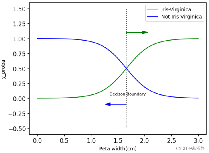
该图表示随着花瓣长度增加该花不属于 Virginica 类型的概率在减小而属于 Virginica 类型的概率在增加
五、决策边界的绘制
步骤如下:
① 构建坐标数据合理的范围当中根据实际训练时输入数据来决定可参考 iris.DESCR
② 整合坐标点得到所有测试输入数据坐标点
③ 预测得到所有点的概率值
④ 绘制等高线完成决策边界
1、训练数据的决策边界
# 为了便于展示通常习惯在二维平面中绘制决策边界其中一个维度是某个属性另一个维度则是另一个属性
# 因此接下来构建分类器时将选取 iris 数据集两个特征
X = iris['data'][:,(2,3)]
print(X.shape)
print(X[:10])

# 这里依然将 Virginica 花的标签设置为 1其余为 0
y = (iris['target']==2).astype(np.int)

# 训练数据
log_res = LogisticRegression()
log_res.fit(X,y)
Out
	(150, 2)
	[[1.4 0.2]
	 [1.4 0.2]
	 [1.3 0.2]
	 [1.5 0.2]
	 [1.4 0.2]
	 [1.7 0.4]
	 [1.4 0.3]
	 [1.5 0.2]
	 [1.4 0.2]
	 [1.5 0.1]]
# 查看标签数据规格和内容
print(y.shape)
y==0
Out
	(150,)
	array([ True,  True,  True,  True,  True,  True,  True,  True,  True,
	        True,  True,  True,  True,  True,  True,  True,  True,  True,
	        True,  True,  True,  True,  True,  True,  True,  True,  True,
	        True,  True,  True,  True,  True,  True,  True,  True,  True,
	        True,  True,  True,  True,  True,  True,  True,  True,  True,
	        True,  True,  True,  True,  True,  True,  True,  True,  True,
	        True,  True,  True,  True,  True,  True,  True,  True,  True,
	        True,  True,  True,  True,  True,  True,  True,  True,  True,
	        True,  True,  True,  True,  True,  True,  True,  True,  True,
	        True,  True,  True,  True,  True,  True,  True,  True,  True,
	        True,  True,  True,  True,  True,  True,  True,  True,  True,
	        True, False, False, False, False, False, False, False, False,
	       False, False, False, False, False, False, False, False, False,
	       False, False, False, False, False, False, False, False, False,
	       False, False, False, False, False, False, False, False, False,
	       False, False, False, False, False, False, False, False, False,
	       False, False, False, False, False, False])
# 构建坐标数据时可参考训练数据集中 X 数组的取值范围
print("训练数组中X[,0]的最小值为 {}最大值为 {}".format(X[:,0].min(),X[:,0].max()))
print("训练数组中X[,1]的最小值为 {}最大值为 {}".format(X[:,1].min(),X[:,1].max()))
Out
	训练数组中X[,0]的最小值为 1.0最大值为 6.9
	训练数组中X[,1]的最小值为 0.1最大值为 2.5
# 构建坐标数据
# meshgrid(ary1, ary2,…, aryN)函数被用于返回 N 组不同的数据以构建 N 维数组其规则如下:
# 1、传入的数组个数有多少个就返回多少个 ndarray;
# 2、传入的数组个数有多少个每个返回的 ndarray 就是多少维的;
# 3、若 ary1 长度为 L1ary2 长度为 L2…aryN 长度为 LN则每个 ndarray 在其每个维度上的长度分别也为 LN、…、L2、L1。
# 4、第 i 个 ndarray 的取值范围即为第 i 个 aryi 。
# 接下来可使用 ravel() 函数来将 N 个 ndarray 拉平然后再用这 N 个数组构建一个 N 维数组。
x0,x1 = np.meshgrid(np.linspace(1.5,7,500).reshape(-1,1),np.linspace(0.5,2.7,200).reshape(-1,1))
X_new = np.c_[x0.ravel(),x1.ravel()]
# 预测
y_proba = log_res.predict_proba(X_new)
# 绘图
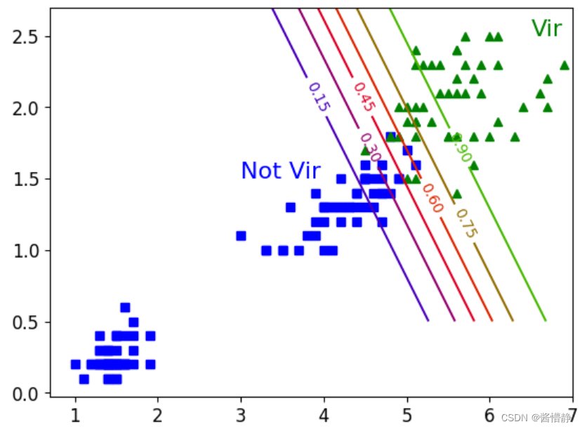
plt.plot(X[y==0,0],X[y==0,1],'bs')
plt.plot(X[y==1,0],X[y==1,1],'g^')
# 查看等高线
zz = y_proba[:,1].reshape(x0.shape)
# 画等高线
contour = plt.contour(x0,x1,zz,cmap=plt.cm.brg)
plt.clabel(contour)
plt.text(3,1.5,'Not Vir',fontsize = 16, color = 'b')
plt.text(6.5,2.5,'Vir',fontsize = 16, color = 'g')
2、测试数据的决策边界
构建坐标棋盘这里需要用到一个函数:meshgrid
meshgrid (ary1, ary2,…, aryN) 函数被用于返回 N 组不同的数据以构建 N 维数组其规则如下:
① 传入的数组个数有多少个就返回多少个 ndarray;
② 传入的数组个数有多少个每个返回的 ndarray 就是多少维的;
③ 若 ary1 长度为 L1ary2 长度为 L2…aryN 长度为 LN则每个 ndarray 在其每个维度上的长度分别也为 L1、L2、…、LN。
④ 第 i 个 ndarray 的取值范围即为第 i 个 aryi 。
接下来可使用 ravel() 函数来将 N 个 ndarray 拉平然后再用这 N 个数组构建一个 N 维数组。
数组拉伸函数说明
numpy.c_(ary1, ary2) :将切片对象沿第二个轴按列连接。
numpy.r_(ary1, ary2) :将切片对象沿第一个轴按行连接。
# 构建两个维度的数据
x0,x1 = np.meshgrid(np.linspace(1.5,7,500),np.linspace(0.5,2.7,200))
# 将两个维度的数据拉伸后进行连接
X_new = np.c_[x0.ravel(),x1.ravel()]
# 可以将以上两个步骤视为对两个数组进行了笛卡尔积操作以此完成数据集的构建
# 计算构建的坐标数据的概率值
y_proba = log_res.predict_proba(X_new)
# 绘图
plt.figure(figsize=(6,4))
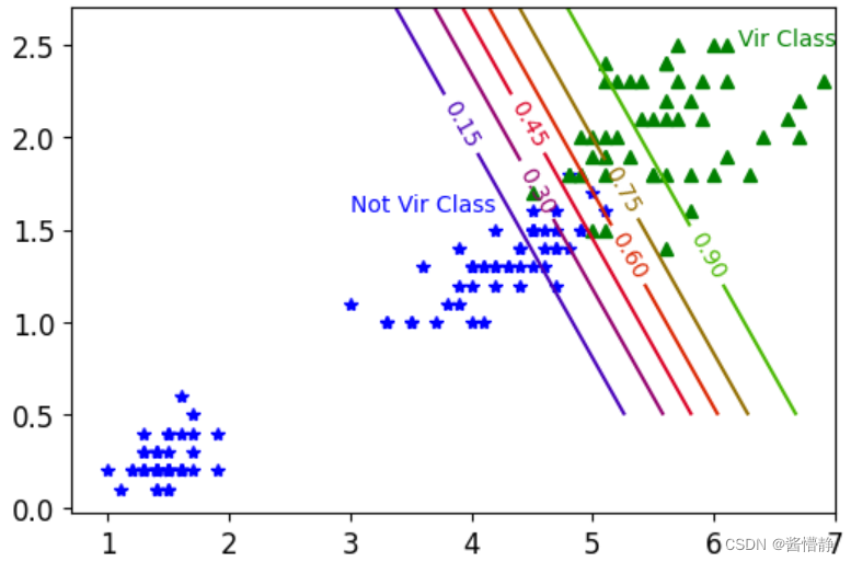
plt.plot(X[y==0,0],X[y==0,1],'b*')
plt.plot(X[y==1,0],X[y==1,1],'g^')
# 得到“z 轴”的线这一步需要 reshape
# 因为 x0x1 是规格为 (200, 500) 的二维数组我们绘制等高线时对于该二维数组中的每个数据都需要画出对应在 z 轴上的线
zz = y_proba[:,1].reshape(x0.shape)
# 设置轮廓等高线的参数
contour = plt.contour(x0,x1,zz,cmap=plt.cm.brg)
# 绘制轮廓等高线
plt.clabel(contour)
# 添加必要的文本内容
plt.text(3,1.6,'Not Vir Class',fontsize = 10, color = 'b')
plt.text(6.2,2.5,'Vir Class',fontsize = 10, color = 'g')
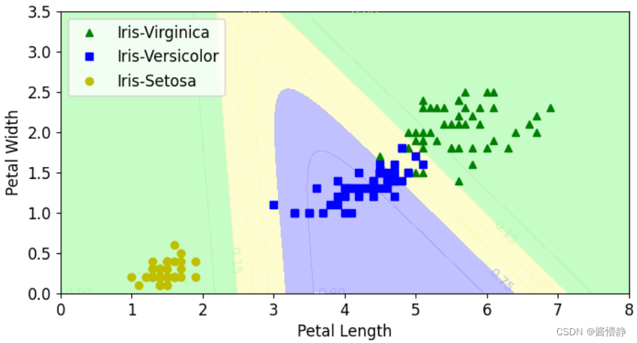
六、多分类实验:softmax
# 构建训练集
X = iris['data'][:,(2,3)]
y = iris['target']

# 多分类:在逻辑回归中加入必要的 multi_class 参数和需要选用的 solver用于优化损失函数的算法
softmax_reg = LogisticRegression(multi_class = 'multinomial',solver = 'lbfgs')
softmax_reg.fit(X,y)

# 调用分类器预测指定的随机数据
softmax_reg.predict_proba([[5,2]])
Out
	array([[2.43559894e-04, 2.14859516e-01, 7.84896924e-01]])
上面的结果给出了对输入向量在三个类别上的概率值。
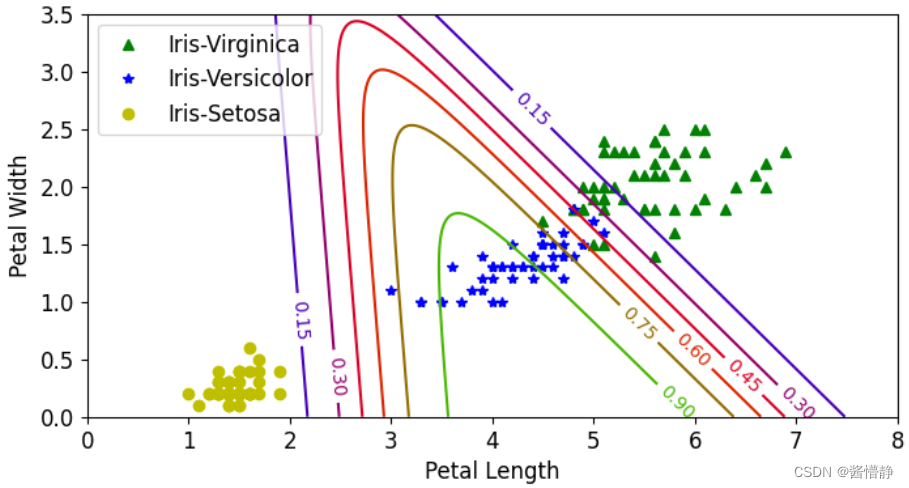
绘制多分类的决策边界
# 构建数据坐标网格点坐标矩阵
x0,x1 = np.meshgrid(
    np.linspace(0,8,500).reshape(-1,1),
    np.linspace(0,3.5,200).reshape(-1,1))
X_new = np.c_[x0.ravel(),x1.ravel()]

y_proba = softmax_reg.predict_proba(X_new)

zz = y_proba[:,1].reshape(x0.shape)

plt.figure(figsize = (8,4))
plt.plot(X[y==2,0],X[y==2,1],'g^',label="Iris-Virginica")
plt.plot(X[y==1,0],X[y==1,1],'bs',label="Iris-Versicolor")
plt.plot(X[y==0,0],X[y==0,1],'yo',label="Iris-Setosa")

from matplotlib.colors import ListedColormap
custom_cmap = ListedColormap(['#a0faa0','#fafab0','#9898ff'])

# alpha 为透明度
contour = plt.contourf(x0,x1,zz,alpha=0.6,cmap = custom_cmap)
plt.clabel(contour,inline = 1,fontsize = 10)
plt.xlim(x0.min(),x0.max())
plt.ylim(x1.min(),x1.max())
plt.xlabel('Petal Length',fontsize = 12)
plt.ylabel('Petal Width',fontsize = 12)
plt.legend(fontsize = 12)
plt.show()
# 构建数据坐标网格点坐标矩阵
x0,x1 = np.meshgrid(
    np.linspace(0,8,500).reshape(-1,1),
    np.linspace(0,3.5,200).reshape(-1,1))
X_new = np.c_[x0.ravel(),x1.ravel()]

y_proba = softmax_reg.predict_proba(X_new)

zz = y_proba[:,1].reshape(x0.shape)

plt.figure(figsize = (8,4))
plt.plot(X[y==2,0],X[y==2,1],'g^',label="Iris-Virginica")
plt.plot(X[y==1,0],X[y==1,1],'b*',label="Iris-Versicolor")
plt.plot(X[y==0,0],X[y==0,1],'yo',label="Iris-Setosa")

from matplotlib.colors import ListedColormap
custom_cmap = ListedColormap(['#a0ffa0','#faffb0','#9899ff'])

contour = plt.contour(x0,x1,zz,cmap = plt.cm.brg)
plt.clabel(contour,inline = 1,fontsize = 10)
plt.xlim(x0.min(),x0.max())
plt.ylim(x1.min(),x1.max())
plt.xlabel('Petal Length',fontsize = 12)
plt.ylabel('Petal Width',fontsize = 12)
plt.legend(fontsize = 12)
plt.show()