大数据分析-实验八鸢尾花数据集分类

阿里云国内75折回扣微信号：monov8

阿里云国际，腾讯云国际，低至75折。AWS 93折免费开户实名账号代冲值优惠多多微信号：monov8 飞机：@monov6

Tec8-鸢尾花数据集分类

1. 使用Sklearn的逻辑回归完成鸢尾花分类预测

# -*- coding: utf-8 -*-
from sklearn.datasets import load_iris
from sklearn.model_selection import train_test_split
from sklearn.linear_model import LogisticRegression

class MyLogicRegression():
    def __init__(self):
        self.iris = load_iris()

    def run(self):
        x_train = self.iris.data
        y_train = self.iris.target
        x_train, x_test, y_train, y_test = train_test_split(x_train, y_train,
                                                            test_size=0.2,
                                                            random_state=0,
                                                            stratify=y_train)
        # logitic 回归的分类模型
        lr = LogisticRegression()
        lr.fit(x_train, y_train)

        result = lr.predict(x_test)
        print('预测的结果', result)
        print('实际的结果', y_test)

if __name__ == '__main__':
    my_logic_regression = MyLogicRegression()
    my_logic_regression.run()

2. 使用BPNN完成鸢尾花数据集分类

# -*- coding: utf-8 -*-
import pandas as pd
import numpy as np
from sklearn.datasets import load_iris

def get_data(name):
    '''
    获取数据
    :param name: 文件名
    :return:x, y
    '''
    data_sets = pd.read_csv(name, header=None)
    x = data_sets.iloc[:, 0:4].values.T
    y = data_sets.iloc[:, 4:].values.T
    y = y.astype("uint8")
    return x, y

'''
构建一个具有1个隐藏层的神经网络，隐层的大小为10
输入层为4个特征，输出层为3个分类
(1,0,0)为第一类，(0,1,0)为第二类，(0,0,1)为第三类
'''
class MyBPNN():
    def __init__(self, epochs, n_hide, n_input, n_output, learning_rate):
        '''
        初始化BP神经网络
        :param epochs: 总训练次数
        :param n_hide: 隐层节点数量
        :param n_input: 输入层节点数量
        :param n_output: 输出层节点数量
        :param learning_rate: 学习率
        '''
        self.epochs = epochs
        self.n_hide = n_hide
        self.n_input = n_input
        self.n_output = n_output
        self.learning_rate = learning_rate

    def _initialize_parameters(self):
        '''
        初始化权重和偏置矩阵
        :return:
        '''
        # 保证随机数一定
        np.random.seed(2)

        self.w1 = np.random.randn(self.n_hide, self.n_input) * 0.01
        self.b1 = np.zeros(shape=(self.n_hide, 1))
        self.w2 = np.random.randn(self.n_output, self.n_hide) * 0.01
        self.b2 = np.zeros(shape=(self.n_output, 1))

    def _forward_propagation(self):
        '''
        前向传播计算a2
        :return:
        '''
        self.z1 = np.dot(self.w1 , self.x_train) + self.b1
        # 使用tanh作为第一层激活函数
        self.a1 = np.tanh(self.z1)
        self.z2 = np.dot(self.w2, self.a1) + self.b2
        # 使用sigmoid作为第二层激活函数
        self.a2 = 1 / (1 + np.exp(-self.z2))

    def _compute_cost(self):
        '''
        计算代价函数
        :return:
        '''

        # 使用交叉熵作为代价函数，交叉熵要求必须满足分布在[0-1]之间
        log = np.multiply(np.log(self.a2), self.y_train) + np.multiply((1 - self.y_train), np.log(1 - self.a2))
        self.cost = - np.sum(log) / self.number

    def _backward_propagation(self):
        '''
        反向传播(计算代价函数的导数)
        :return:
        '''
        self.dz2 = self.a2 - self.y_train
        self.dw2 = (1 / self.number) * np.dot(self.dz2, self.a1.T)
        self.db2 = (1 / self.number) * np.sum(self.dz2, axis=1, keepdims=True)

        self.dz1 = np.multiply(np.dot(self.w2.T, self.dz2), 1 - np.power(self.a1, 2))
        self.dw1 = (1 / self.number) * np.dot(self.dz1, self.x_train.T)
        self.db1 = (1 / self.number) * np.sum(self.dz1, axis=1, keepdims=True)

    def _update_param(self):
        self.w1 = self.w1 - self.dw1 * self.learning_rate
        self.b1 = self.b1 - self.db1 * self.learning_rate
        self.w2 = self.w2 - self.dw2 * self.learning_rate
        self.b2 = self.b2 - self.db2 * self.learning_rate

    def fit(self, x_train, y_train, print_cost = True):
        # 保证随机数一定
        np.random.seed(3)

        # 加载数据
        self.x_train = x_train
        self.y_train = y_train
        self.number = self.y_train.shape[1]

        # 初始化参数
        self._initialize_parameters()

        # 执行梯度下降循环
        for i in range(0, self.epochs):
            # 前向传播
            self._forward_propagation()
            # 计算代价
            self._compute_cost()
            # 反向传播
            self._backward_propagation()
            # 更新参数
            self._update_param()

            if(print_cost and ((i % 1000) == 0)):
                print('迭代第%i次，代价为：%f' % (i, self.cost))

    def predict(self, x_test, y_test):
        '''
        预测结果
        :param x_test:
        :param y_test:
        :return:
        '''
        # 进行正向传播
        z1 = np.dot(self.w1, x_test) + self.b1
        a1 = np.tanh(z1)
        z2 = np.dot(self.w2, a1) + self.b2
        a2 = 1 / (1 + np.exp(-z2))

        # 结果的维度
        n_rows = y_test.shape[0]
        n_cols = y_test.shape[1]

        # 预测值结果存储
        output = np.empty(shape=(n_rows, n_cols), dtype=int)

        for i in range(n_rows):
            for j in range(n_cols):
                if a2[i][j] > 0.5:
                    output[i][j] = 1
                else:
                    output[i][j] = 0

        # print('预测结果：')
        # print(output)
        # print('真实结果：')
        # print(y_test)

        count = 0
        for k in range(0, n_cols):
            if output[0][k] == y_test[0][k] and output[1][k] == y_test[1][k] and output[2][k] == y_test[2][k]:
                count = count + 1
            else:
                # print(k)
                continue

        acc = count / int(y_test.shape[1]) * 100
        print('测试集准确率：%.2f%%' % acc)

        return output

if __name__ == '__main__':
    iris = load_iris()
    x_train, y_train = get_data('../Datasets/iris-train.csv')
    x_test, y_test = get_data('../Datasets/iris-test.csv')

    my_bpnn = MyBPNN(10000, 10, 4, 3, 0.4)
    my_bpnn.fit(x_train, y_train)
    result = my_bpnn.predict(x_test, y_test)

3. 决策树实现鸢尾花数据集分类

决策树的每一个叶节点的实例都属于同一类
决策树算法的最大特点是可以自学习
建立决策树的主要算法有

ID3算法:信息增益
C4.5算法:信息增益率
CART算法:Gini系数

3.1. Sklearn提供的DecisionTreeClassifier

大数据分析-实验八鸢尾花数据集分类_sklearn

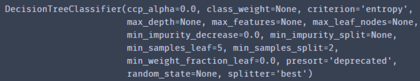
DecisionTreeClassifier():是用来创建一个决策树模型

criterion

gini:基尼系数
entropy:信息熵。

splitter：

best 是在所有特征中找最好的切分点
random后者是在部分特征中找最好的切分点
默认的best适合样本量不大的时候，而如果样本数据量非常大，此时决策树构建推荐random 。

max_features

None(所有)
log2
sqrt
特征小于50的时候一般使用所有的特征进行训练

max_depth

None(默认)
整数:设置决策随机森林中的决策树的最大深度，深度越大，越容易过拟合，推荐树的深度为：5-20之间。

min_samples_split：设置结点的最小样本数量，当样本数量可能小于此值时，结点将不会在划分。
min_samples_leaf：这个值限制了叶子节点最少的样本数，如果某叶子节点数目小于样本数，则会和兄弟节点一起被剪枝。
min_weight_fraction_leaf：这个值限制了叶子节点所有样本权重和的最小值，如果小于这个值，则会和兄弟节点一起被剪枝默认是0，就是不考虑权重问题。
max_leaf_nodes：通过限制最大叶子节点数，可以防止过拟合，默认是None，即不限制最大的叶子节点数。
class_weight：指定样本各类别的的权重，主要是为了防止训练集某些类别的样本过多导致训练的决策树过于偏向这些类别。这里可以自己指定各个样本的权重，如果使用balanced，则算法会自己计算权重，样本量少的类别所对应的样本权重会高。
min_impurity_split：这个值限制了决策树的增长，如果某节点的不纯度(基尼系数，信息增益，均方差，绝对差)小于这个阈值则该节点不再生成子节点。即为叶子节点。

3.2. sklearn的决策树的自带可视化

plt.figure(figsize=(8, 8))
tree.plot_tree(clf, filled='True',
            feature_names=['花萼长', '花萼宽', '花瓣长', '花瓣宽'],
            class_names=['山鸢尾', '变色鸢尾', '维吉尼亚鸢尾'])
plt.savefig("./Flower_Tree.png", bbox_inches="tight", pad_inches=0.0)

3.3. sklearn的决策树的加载

# 仅供示例
from sklearn import tree

f = open('../dataSet/iris_tree.dot', 'w')
tree.export_graphviz(model.get_params('DTC')['DTC'], out_file=f)

3.4. 全部代码

# -*- coding: utf-8 -*-
from sklearn.datasets import load_iris
from sklearn.model_selection import train_test_split
from sklearn import tree
import matplotlib
from matplotlib import pyplot as plt

# 配置全局的matplotlib参数
matplotlib.rcParams['font.family'] = 'SimHei'
matplotlib.rcParams['axes.unicode_minus'] = False

class MyDecisionTree():
    def __init__(self, criterion, splitter, max_depth, min_samples_split):
        self.iris = load_iris()
        self.criterion = criterion
        self.splitter = splitter
        self.max_depth = max_depth
        self.min_samples_split = min_samples_split

    def run(self):
        x_train = self.iris.data
        y_train = self.iris.target
        x_train, x_test, y_train, y_test = train_test_split(x_train, y_train,
                                                            test_size=0.2,
                                                            random_state=0,
                                                            stratify=y_train)
        clf = tree.DecisionTreeClassifier(criterion=self.criterion, splitter=self.splitter
                                          , max_depth=self.max_depth
                                          , min_samples_split=self.min_samples_split)
        clf.fit(x_train, y_train)

        print("模型参数:")
        print(" criterion:" + self.criterion)
        print(" splitter:" + self.splitter)
        print(" max_depth:" + str(self.max_depth))
        print(" min_samples_split:" + str(self.min_samples_split))

        # 训练集准确率
        result = clf.predict(x_train)
        true_number = 0
        total_number = y_train.shape[0]
        for x, y in zip(result, y_train):
            if (x == y):
                true_number += 1
        print("训练集准确率:", true_number / total_number * 1.0)

        # 测试集准确率
        result = clf.predict(x_test)
        true_number = 0
        total_number = y_test.shape[0]
        for x,y in zip(result, y_test):
            if(x == y):
                true_number += 1
        print("测试集准确率:", true_number / total_number * 1.0)

        plt.figure(figsize=(8, 8))
        tree.plot_tree(clf, filled='True',
                       feature_names=['花萼长', '花萼宽', '花瓣长', '花瓣宽'],
                       class_names=['山鸢尾', '变色鸢尾', '维吉尼亚鸢尾'])
        plt.savefig("./Flower_Tree.png", bbox_inches="tight", pad_inches=0.0)

if __name__ == '__main__':
    my_decision_tree = MyDecisionTree(
        "gini", "best", 4, 2)
    my_decision_tree.run()

4. SVM实现鸢尾花数据集分类

4.1. 使用SKlearn中自带的SVM中的SVC

sklearn.svm.SVC(C=1.0, kernel='rbf', degree=3, gamma='auto', coef0=0.0, shrinking=True, probability=False,tol=0.001, cache_size=200, class_weight=None, verbose=False, max_iter=-1, decision_function_shape=None,random_state=None)

C:C-SVC的惩罚参数，默认值为1.0，C相当于惩罚松弛变量

C值大，即对误分类的惩罚增大，趋向于对训练集圈粉对的情况，这样对训练集的测试准确率更高，但泛化能力弱。
C值小，对误分类的惩罚减小，允许出错化将他们作为噪声点，泛化能力较强。

decision_function_shape：决策函数形状

None
ovo:one versus one, 一对一的分类器，这时对于K个类别需要构建 $大数据分析-实验八鸢尾花数据集分类_数据分析_02$ 个分类器
ovr:one versus rest, 一对其他的分类器，这时对K个类别只需要构建K个分类器

kernel:核函数，默认为rbf

rbf:高斯核函数
poly:多项式核函数
linear:线性核函数
sigmoid:sigmoid函数

degree:如果选择多项式核函数poly，默认是3，选择其他核函数时会被忽略。
gamma:高斯核函数、多项式核函数和sigmoid核函数的参数，默认是auto
coef0:核函数的常数项，对于多项式核函数和sigmoid有效
probability:是否采用概率估计，默认为False
shrinking:是否使用shrinking heuristic(启发式收缩)，默认为True
tol:停止训练的误差大小，默认为1e-3
cache_size:核函数cache缓存大小，默认为200
class_weight:类别的权重，字段形式传递，设置第几类的参数C为weight * C
verbose:是否允许冗余输出
max_iter:最大迭代次数，-1为无限制
random_state:数据洗牌时的种子值，int

SVC参数官方文档

4.2. 完整代码

# -*- coding: utf-8 -*-
from sklearn.datasets import load_iris
from sklearn.model_selection import train_test_split
from sklearn import svm

class MySVM():
    def __init__(self):
        self.iris = load_iris()

    def run(self, kernel, C):
        x_train = self.iris.data
        y_train = self.iris.target
        x_train, x_test, y_train, y_test = train_test_split(x_train, y_train,
                                                            test_size=0.2,
                                                            random_state=0,
                                                            stratify=y_train)
        svm_classifier = svm.SVC(C=C, kernel=kernel, decision_function_shape='ovr')
        svm_classifier.fit(x_train, y_train)

        print("核函数:" + kernel + "，惩罚参数:" + str(C))
        print("训练集准确率:", svm_classifier.score(x_train, y_train))
        print("测试集准确率:", svm_classifier.score(x_test, y_test))

if __name__ == '__main__':
    my_svm = MySVM()
    my_svm.run("linear", 1.0)