针对KF状态估计的电力系统虚假数据注入攻击研究（Matlab代码实现）

阿里云国内75折回扣微信号：monov8

阿里云国际，腾讯云国际，低至75折。AWS 93折免费开户实名账号代冲值优惠多多微信号：monov8 飞机：@monov6

欢迎来到本博客❤️❤️

博主优势博客内容尽量做到思维缜密逻辑清晰为了方便读者。

⛳️座右铭行百里者半于九十。

本文目录如下

目录

1 概述

2 运行结果

3 参考文献

4 Matlab代码实现

1 概述

如今现代电力系统正在向智能化方向发展大量的智能设备如智能仪表和传感器促进了电力系统在发电、变电、输电和配电模式方面的转变使得智能电网成为一个典型的网络物理系统即将物理电力传输系统和计算机网络相结合。在智能电网中监督控制和数据采集系统SCADA实时收集外场设备通过网络发送来的数据进行分析后向控制中心汇报收集到的信息控制中心根据这些信息对电网的发电配电进行调整。

在享受智能电网带来便利的同时由于使用了大量智能设备以及通过网络来收发数据使得智能电网更容易遭到攻击者的攻击。最为显著的是通过有预谋地篡改智能设备的数据来达到攻击电力系统的目的称之为虚假数据注入攻击FDIA。为了保障电力服务的平稳运行智能电网的检测至关重要。

FDIA 的攻击目标主要包括测量单元、通信网络和控制设备。由于控制设备往往保护级别较高而难以入侵因此FDIA 通常以前两种方式实施。在实施 FDIA 过程中攻击者首要任务是入侵系统网络。例如为了破坏测量单元例如远程终端单元和向量测量单元的数据攻击者往往利用加密和认证机制固有的漏洞来进行入侵并修改原始数据。在文献[17]中研究人员揭示了通过欺骗向量测量单元全球定位系统的时间同步攻击。由于全球定位系统信号并无加密或授权机制攻击者可以产生伪冒的全球定位系统信号而接收器无法从原始数据中辨别出来。

攻击者在侵入系统网络后可以获得测量修改权限。根据潮流规律某一测量值的变化会引起相邻测量值的变化。当伪造一个数据例如节点或传输线路的测量值时为了绕过坏数据检测攻击者会考虑潮流定律找到测量数据相应改变的最小空间。而将需要协同攻击的最小空间定义为该数据在执行 FDIA 时满足潮流规律和最优资源利用规律的最小相关空间[18]。

状态估计方法分为静态估计和动态估计。传统的电力系统状态估计方法采用的是加权最小二乘估计器等静态估计方法。这是建立在电力系统具有足够冗余且处于稳态状态的假设之上的[8]。然而由于用电需求和发电量是实时变化的因此真实的电力系统并不是在稳定状态下运行[19]。同时静态估计方法仅考虑当前时刻数据没有关联先前的状态因此其估计结果精度不佳。为了解决这些问题动态状态估计器如卡尔曼滤波器被引入电力系统状态估计[20]。接下来讨论了不同的基于状态估计的 FDIA 检测方案其分类如图 3.2 所示。本文选择KF

2 运行结果

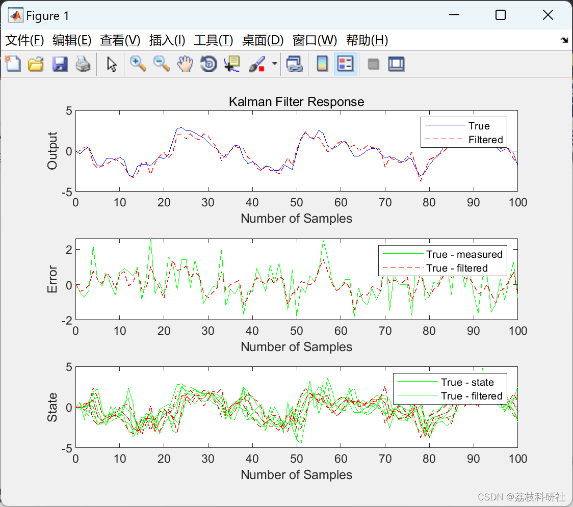
clf
subplot(311), plot(t,yt,'b',t,y_hat,'r--'),
xlabel('Number of Samples'), ylabel('Output')
title('Kalman Filter Response')
legend('True','Filtered')
subplot(312), plot(t,yt-y,'g',t,yt-y_hat,'r--'),
xlabel('Number of Samples'), ylabel('Error')
legend('True - measured','True - filtered')

subplot(313), plot(t, state,'g',t,[x1_hat, x2_hat,x3_hat],'r--'),
xlabel('Number of Samples'), ylabel('State')
legend('True - state','True - filtered')

....

figure;
plot(t, filtered, t, v);
ylim([-2 2]);
xlabel('time (in seconds)');
legA = legend('filtered','real');
set(legA,'FontSize',12)
title('signal vs. estimation');
grid on

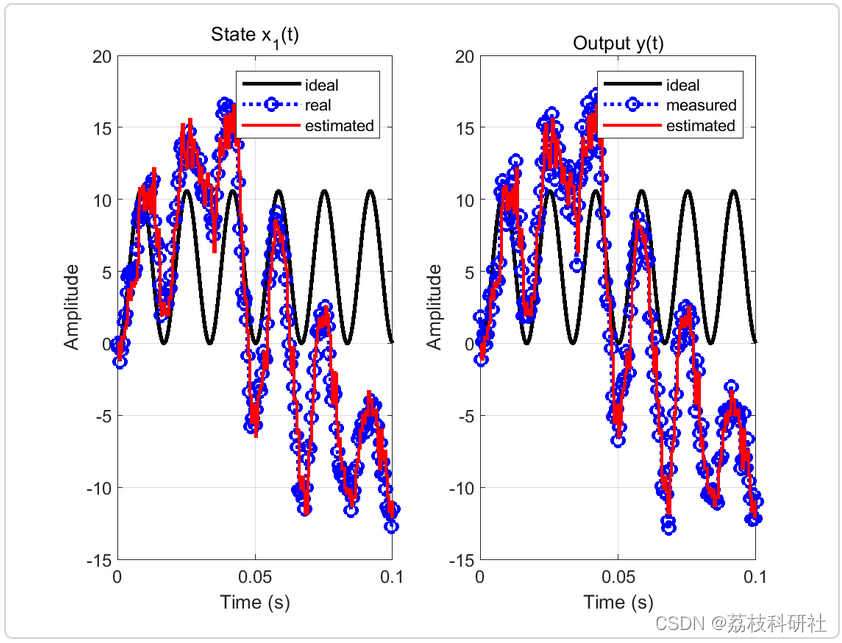
[y_o,t_o,x_o] = lsim( sys, [u 0*w], t); % IDEAL behavior for comparison
figure(1)
for k = 1:length(sys.A)
subplot( round((length(sys.A)+1)/2 ),2,k)
plot(t,x_o(:,k),'k','linewidth',2); hold on;
plot(t,x_(:,k),'bo:','linewidth',2);
stairs(t,x(:,k),'r','linewidth',1.5);
xlabel('Time (s)'); ylabel('Amplitude'); title(['State x_' num2str(k) '(t)']); grid on;
legend('ideal','real','estimated'); hold off;
end
subplot( round((length(sys.A)+1)/2 ),2,k+1)
plot(t,y_o,'k','linewidth',2); hold on;
plot(t,z,'bo:','linewidth',2);
stairs(t,y,'r','linewidth',1.5);
xlabel('Time (s)'); ylabel('Amplitude'); title('Output y(t)'); grid on;
legend('ideal','measured','estimated');

%Generate process noise and sensor noise vectors using the same noise covariance values Q and R that you used to design the filter.
rng(10,'twister');
w1 = sqrt(Q)*randn(length(t),1);
v1 = sqrt(R)*randn(length(t),1);

%Finally, simulate the response using lsim.
out = lsim(SimModel,[u,w1,v1]);
%lsim generates the response at the outputs yt and ye to the inputs applied at w, v, and u. Extract the yt and ye channels and compute the measured response.

yt = out(:,1); % true response
ye = out(:,2); % filtered response
y = yt + v1; % measured response

%Compare the true response with the filtered response.
clf
subplot(211), plot(t,yt,'b',t,ye,'r--'),
xlabel('Number of Samples'), ylabel('Output')
title('Kalman Filter Response')
legend('True','Filtered')
subplot(212), plot(t,yt-y,'g',t,yt-ye,'r--'),
xlabel('Number of Samples'), ylabel('Error')
legend('True - measured','True - filtered')

%covariance of the error before filtering (measurement error covariance)
MeasErr = yt-yt;
MeasErrCov = sum(MeasErr.*MeasErr)/length(MeasErr) %=0
% and after filtering (estimation error covariance)
EstErr = yt-ye;
EstErrCov = sum(EstErr.*EstErr)/length(EstErr)
% so the Kalman filter reduces the error yt - y due to measurement noise

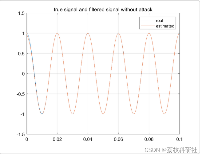
% Kalman filter
[y_hat, ~, ~, P_last, K_last, x_hat, K_steps, P_steps] = kalmanfilter(y, Q, R, StopTime);

e_real = x - x_hat; %state error

figure();
plot(t,y, t, y_hat);
ylim([-1.5,1.5]);
legA = legend('real','estimated');
title('true signal and filtered signal without attack');grid on;