唐宇迪机器学习实战课程笔记(全)
| 阿里云国内75折 回扣 微信号:monov8 |
| 阿里云国际,腾讯云国际,低至75折。AWS 93折 免费开户实名账号 代冲值 优惠多多 微信号:monov8 飞机:@monov6 |
机器学习模型的参数不是直接数学求解而是利用数据进行迭代epoch梯度下降优化求解。
1. 线性回归
1.1线性回归理论
-
目标更好的拟合连续函数(分割连续样本空间的平面h(·))

-
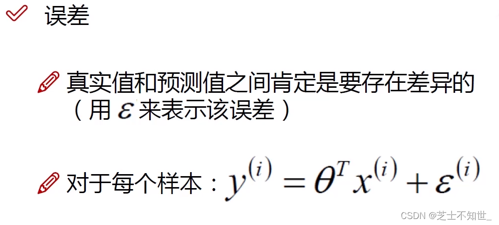
ε ( i ) \varepsilon^{(i)} ε(i)是 真实值 y ( i ) y^{(i)} y(i) 与 预测值 h θ ( x ) = θ T x ( i ) h_\theta (x)=\theta^Tx^{(i)} hθ(x)=θTx(i)之间的误差
-
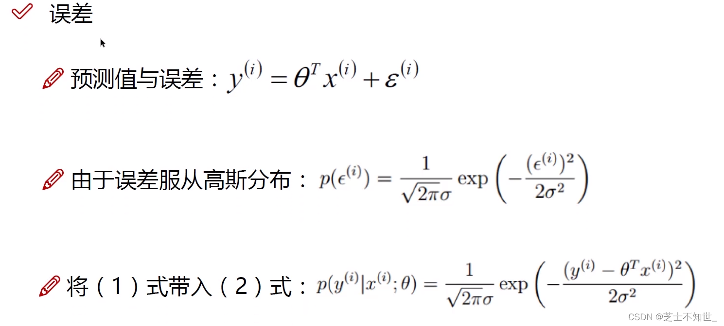
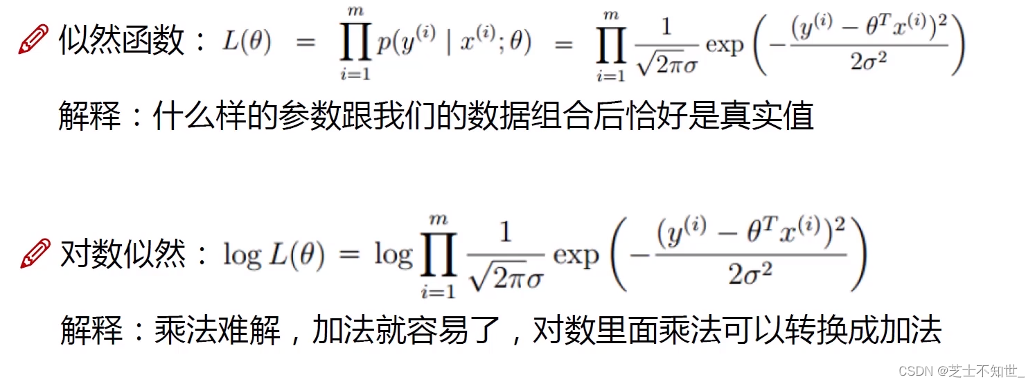
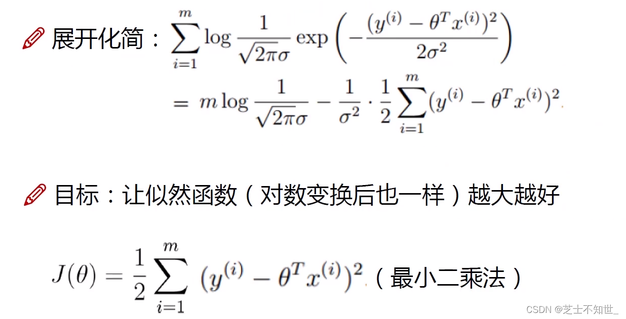
求解参数 θ \theta θ 误差项 ε \varepsilon ε服从高斯分布利用最大似然估计转换为最小二乘法
-
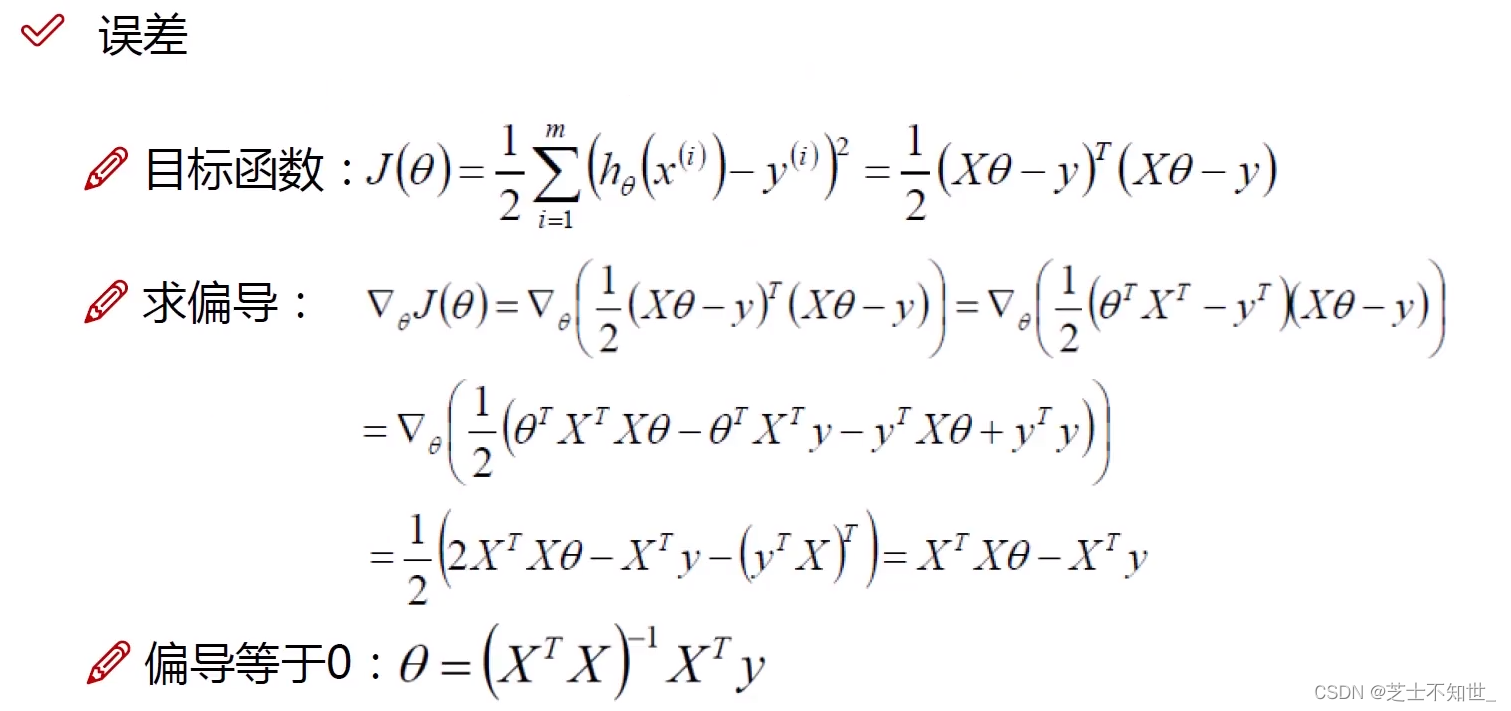
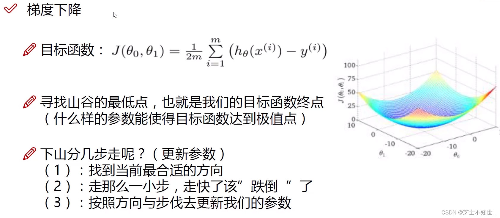
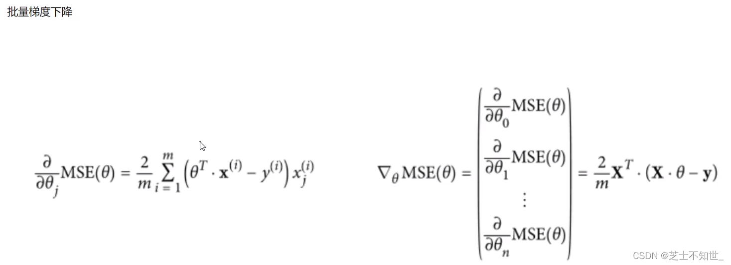
从最小二乘法得到目标函数 J ( θ ) J(\theta) J(θ)为求其最值利用梯度下降算法沿偏导数(梯度)反方向迭代更新计算求解参数 θ \theta θ 。
-
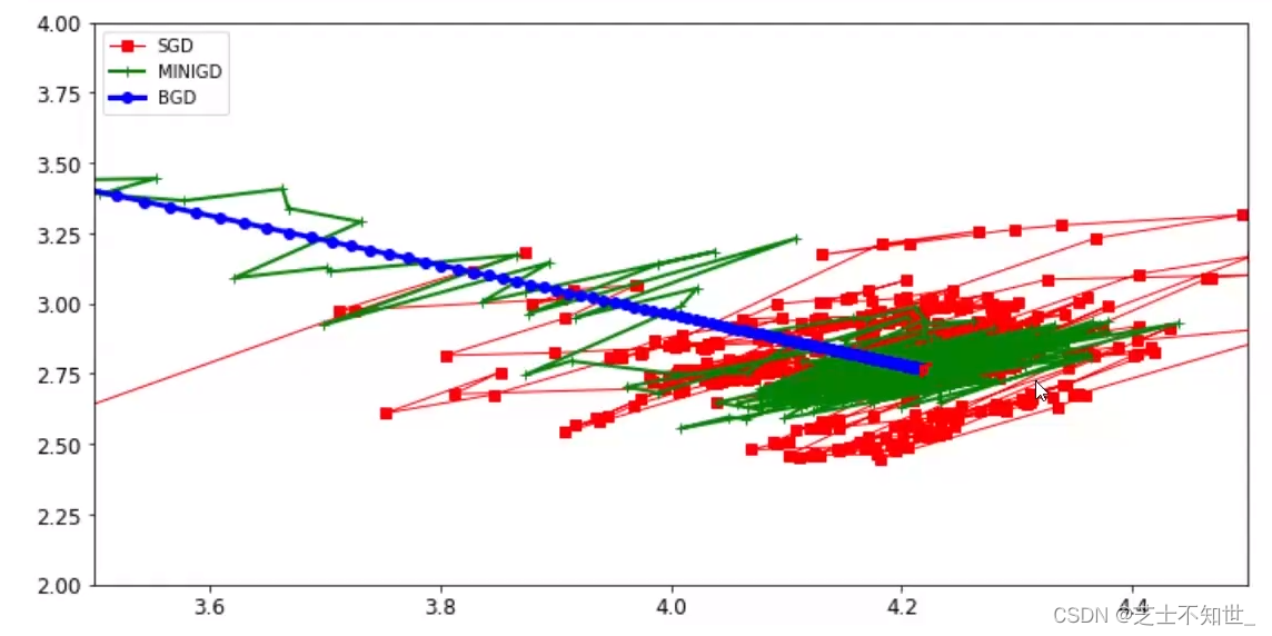
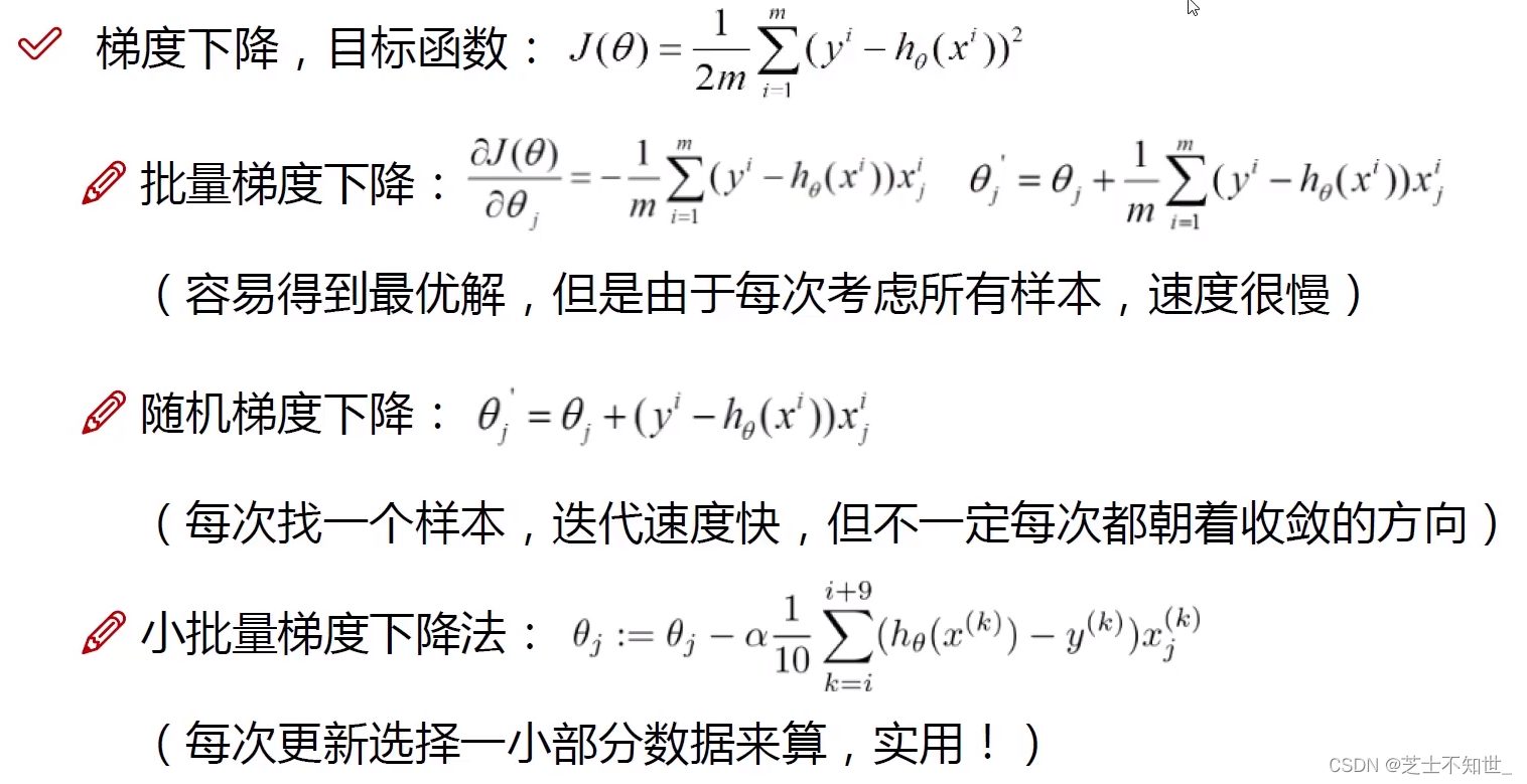
梯度下降算法BatchGD批量梯度下降、SGD随机梯度下降、Mini-BatchGD小批量梯度下降(实用)
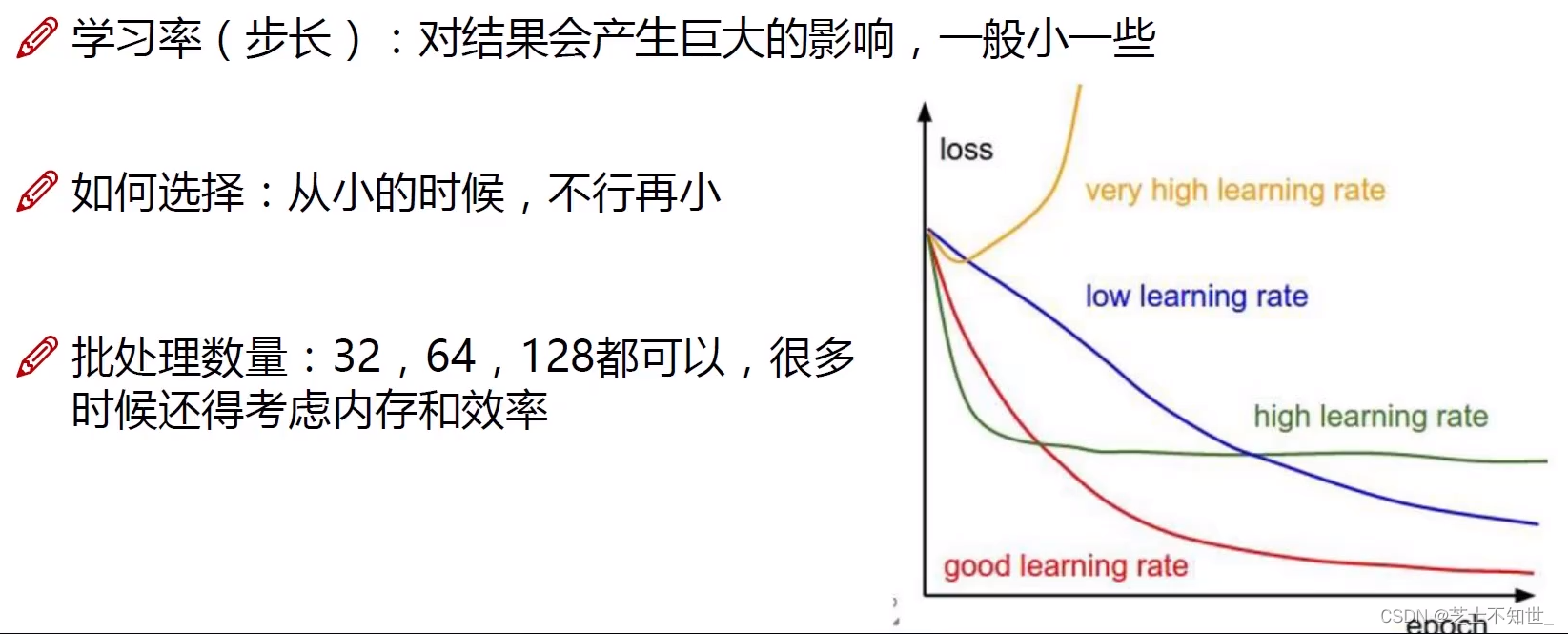
batch一般设为 2 5 2^5 25=64、 2 6 2^6 26=128、 2 7 2^7 27=256越大越好
GD的矩阵运算
-
学习率lr开始设1e-3逐渐调小到1e-5
1.2线性回归实战
数据预处理中normalize标准化作用对输入全部数据 X − μ σ \frac{ X-\mu}{\sigma } σX−μ使得不同值域的输入 x i x_i xi、 x j x_j xj分布在同一取值范围。如 x i ∈ [ 0.1 , 0.5 ] x_i\in[0.1, 0.5] xi∈[0.1,0.5] x j ∈ [ 10 , 50 ] x_j\in[10, 50] xj∈[10,50]normalize使其同一值域。
prepare__for_train.py
"""Prepares the dataset for training"""

import numpy as np
from .normalize import normalize
from .generate_sinusoids import generate_sinusoids
from .generate_polynomials import generate_polynomials


def prepare_for_training(data, polynomial_degree=0, sinusoid_degree=0, normalize_data=True):

    # 计算样本总数
    num_examples = data.shape[0]

    data_processed = np.copy(data)

    # 预处理
    features_mean = 0
    features_deviation = 0
    data_normalized = data_processed
    if normalize_data:
        (
            data_normalized,
            features_mean,
            features_deviation
        ) = normalize(data_processed)

        data_processed = data_normalized

    # 特征变换sinusoidal
    if sinusoid_degree > 0:
        sinusoids = generate_sinusoids(data_normalized, sinusoid_degree)
        data_processed = np.concatenate((data_processed, sinusoids), axis=1)

    # 特征变换polynomial
    if polynomial_degree > 0:
        polynomials = generate_polynomials(data_normalized, polynomial_degree, normalize_data)
        data_processed = np.concatenate((data_processed, polynomials), axis=1)

    # 加一列1
    data_processed = np.hstack((np.ones((num_examples, 1)), data_processed))

    return data_processed, features_mean, features_deviation
linearRegressionClass.py
class LinearRegression_:

    def __init__(self, data, labels, polynomial_degree=0, sinusoid_degree=0, normalize_data=True):
        """
        1.对数据进行预处理操作
        2.先得到所有的特征个数
        3.初始化参数矩阵
        """
        (data_processed,
         features_mean,
         features_deviation) = prepare_for_training(data, polynomial_degree, sinusoid_degree, normalize_data=True)

        self.data = data_processed
        self.labels = labels
        self.features_mean = features_mean
        self.features_deviation = features_deviation
        self.polynomial_degree = polynomial_degree
        self.sinusoid_degree = sinusoid_degree
        self.normalize_data = normalize_data

        num_features = self.data.shape[1]
        self.theta = np.zeros((num_features, 1))

    def train(self, alpha=0.01, num_iterations=500):
        """
                    训练模块执行梯度下降
        """
        cost_history = self.gradient_descent(alpha, num_iterations)
        return self.theta, cost_history

    def gradient_descent(self, alpha, num_iterations):
        """
                    实际迭代模块会迭代num_iterations次
        """
        cost_history = []
        for _ in range(num_iterations):
            self.gradient_step(alpha)
            cost_history.append(self.cost_function(self.data, self.labels))
        return cost_history

    def gradient_step(self, alpha):
        """
                    梯度下降参数更新计算方法注意是矩阵运算
        """
        num_examples = self.data.shape[0]
        prediction = LinearRegression_.hypothesis(self.data, self.theta)
        delta = prediction - self.labels
        theta = self.theta
        theta = theta - alpha * (1 / num_examples) * (np.dot(delta.T, self.data)).T
        self.theta = theta

    def cost_function(self, data, labels):
        """
                    损失计算方法
        """
        num_examples = data.shape[0]
        delta = LinearRegression_.hypothesis(self.data, self.theta) - labels
        cost = (1 / 2) * np.dot(delta.T, delta) / num_examples
        return cost[0][0]

    @staticmethod
    def hypothesis(data, theta):
        predictions = np.dot(data, theta)
        return predictions

    def get_cost(self, data, labels):
        data_processed = prepare_for_training(data,
                                              self.polynomial_degree,
                                              self.sinusoid_degree,
                                              self.normalize_data
                                              )[0]

        return self.cost_function(data_processed, labels)

    def predict(self, data):
        """
                    用训练的参数模型与预测得到回归值结果
        """
        data_processed = prepare_for_training(data,
                                              self.polynomial_degree,
                                              self.sinusoid_degree,
                                              self.normalize_data
                                              )[0]

        predictions = LinearRegression_.hypothesis(data_processed, self.theta)

        return predictions
单输入变量线性回归
y
=
θ
1
x
1
+
b
y=\theta^1x^1+b
y=θ1x1+b
single_variate_LinerRegression.py
import os
import numpy as np
import matplotlib.pyplot as plt
import pandas as pd
from linearRegressionClass import *
dirname = os.path.dirname(__file__)
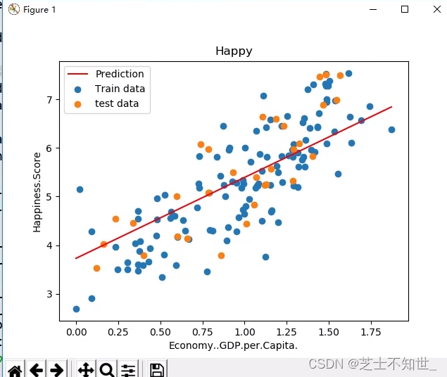
data = pd.read_csv(dirname + "/data/world-happiness-report-2017.csv", sep=',')
train_data = data.sample(frac=0.8)
test_data = data.drop(train_data.index)
# 选定考虑的特征
input_param_name = 'Economy..GDP.per.Capita.'
output_params_name = 'Happiness.Score'
x_train = train_data[[input_param_name]].values
y_train = train_data[[output_params_name]].values
x_test = test_data[[input_param_name]].values
y_test = test_data[[output_params_name]].values
# 用创建的随机样本测试
# 构造样本的函数
# def fun(x, slope, noise=1):
# x = x.flatten()
# y = slope*x + noise * np.random.randn(len(x))
# return y
# # 构造数据
# slope=2
# x_max = 10
# noise = 0.1
# x_train = np.arange(0,x_max,0.2).reshape((-1,1))
# y_train = fun(x_train, slope=slope, noise=noise)
# x_test = np.arange(x_max/2, x_max*3/2, 0.2).reshape((-1,1))
# y_test = fun(x_test, slope=slope, noise=noise)
# #观察训练样本和测试样本
# # plt.scatter(x_train, y_train, label='train data', c='b')
# # plt.scatter(x_test, y_test, label='test data', c='k')
# # plt.legend()
# # plt.title('happiness - GDP')
# # plt.show()
# #测试 - 与唐宇迪的对比
# lr = LinearRegression()
# lr.fit(x_train, y_train)
# print(lr.predict(x_test))
# print(y_test)
# y_train = y_train.reshape((-1,1))
# lr = LinearRegression_(x_train, y_train)
# lr.train()
# print(lr.predict(x_test))
# print(y_test)
lr = LinearRegression()
lr.fit(x_train, y_train, alpha=0.01, num_iters=500)
y_pre = lr.predict(x_test)
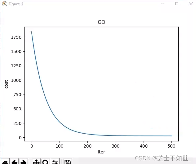
print("开始损失和结束损失", lr.cost_hist[0], lr.cost_hist[-1])
# iters-cost curve
# plt.plot(range(len(lr.cost_hist)), lr.cost_hist)
# plt.xlabel('Iter')
# plt.ylabel('cost')
# plt.title('GD')
# plt.show()
plt.scatter(x_train, y_train, label='Train data')
plt.scatter(x_test, y_test, label='test data')
plt.plot(x_test, y_pre, 'r', label='Prediction')
plt.xlabel(input_param_name)
plt.ylabel(output_params_name)
plt.title('Happy')
plt.legend()
plt.show()
多输入变量线性回归
y
=
∑
i
=
1
n
θ
i
x
i
+
b
y=\sum_{i=1}^{n} \theta^ix^i+b
y=i=1∑nθixi+b
非线性回归
1.对原始数据做非线性变换如
x
−
>
l
n
(
x
)
x->ln(x)
x−>ln(x)
2.设置回归函数的复杂度最高
x
n
x^n
xn
2.分类模型评估(Mnist实战SGD_Classifier)
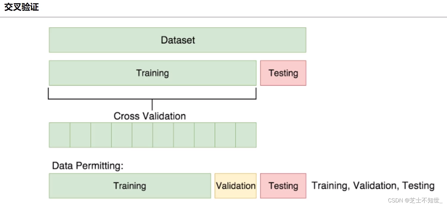
2.1 K折交叉验证K-fold cross validation
①切分完训练集training和测试集testing后
②再对training进行均分为K份
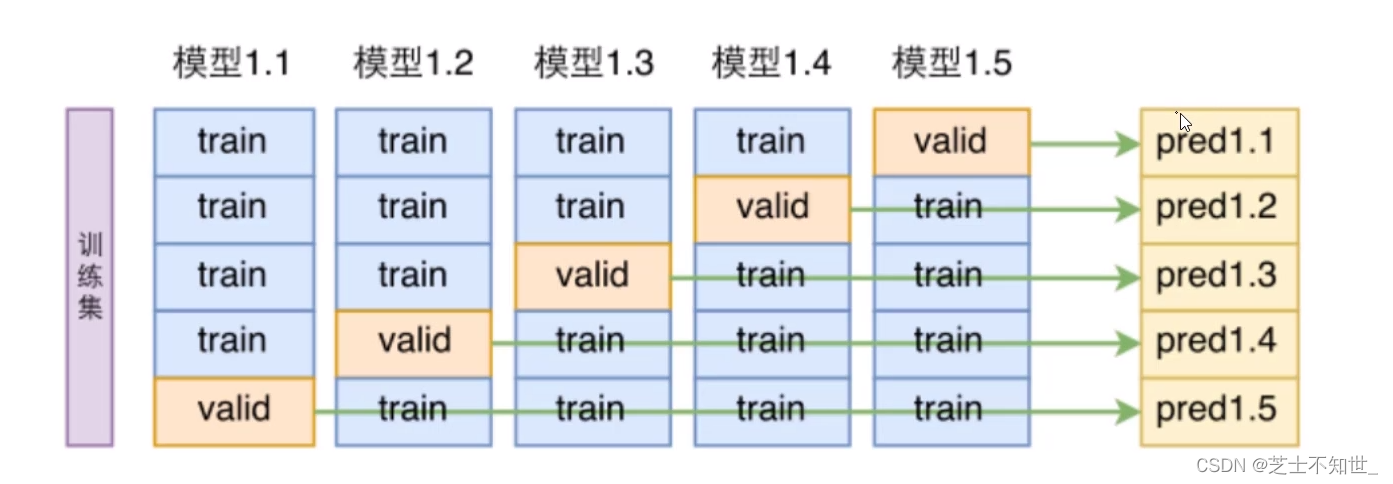
③训练的迭代将进行K轮每轮将其中K-1份作为training1份作为验证机validation边训练train边验证valid
④最后训练和验证的epoch结束了再用测试集testing进行测试。
常用的K=5/10
import numpy as np
import os
import matplotlib
import matplotlib.pyplot as plt

plt.rcParams['axes.labelsize'] = 14
plt.rcParams['xtick.labelsize'] = 12
plt.rcParams['ytick.labelsize'] = 12
import warnings

warnings.filterwarnings('ignore')
np.random.seed(42)

# from sklearn.datasets import fetch_openml
# mnist = fetch_openml('MNIST original')
# 也可以GitHub下载手动加载
import scipy.io

mnist = scipy.io.loadmat('MNIST-original')
# 图像数据 (28x28x1)的灰度图每张图像有784个像素点(=28x28x1)
# print(mnist)  # 字典key=data和label数据存在对应的value中
X, y = mnist['data'], mnist['label']
# print(X.shape)  # data  784 x 70000,每列相当于一张图共70000张图像
# print(y.shape)  # label 1 x 70000共70000个标签


# 划分数据训练集training测试集testingtrain取前60000test取后10000
# 列切片
X_train, X_test, y_train, y_test = X[:, :60000], X[..., 60000:], y[:, :60000], y[..., 60000:]
# 训练集数据洗牌打乱
import numpy as np

X_train = np.random.permutation(X_train)
y_train = np.random.permutation(y_train)

# 因为后面要画混淆矩阵最好是2分类任务0-10的数字判断是不是5
# 将label变为true和false
y_train_5 = (y_train == 5)[0]
y_test_5 = (y_test == 5)[0]

# print(X_train.shape)
# print(y_train_5.shape)

X_train = X_train.T
X_test = X_test.T
# 创建线性模型SGDClassifier
from sklearn.linear_model import SGDClassifier

sgd_clf = SGDClassifier(max_iter=50, random_state=42)
# sgd_clf.fit(X_train, y_train_5)  # 训练
# print(sgd_clf.predict(X_test))

# K折交叉验证 划分训练集training验证集validation并训练

# 方法一
from sklearn.model_selection import cross_val_score
kfold=5
acc=cross_val_score(sgd_clf, X_train, y_train_5, cv=kfold, scoring='accuracy')  ## cv是折数
avg_acc = sum(acc) / kfold
print("avg_acc=", avg_acc)
# 返回每折的acc[0.87558333 0.95766667 0.86525 0.91483333 0.94425]


# 方法二
from sklearn.model_selection import StratifiedKFold
from sklearn.base import clone  # K折中每折训练时模型带有相同参数
kfold = 5
acc = []
skfold = StratifiedKFold(n_splits=kfold, random_state=42)
i = 1
for train_idx, test_idx in skfold.split(X_train, y_train_5):
    # 克隆模型
    clone_clf = clone(sgd_clf)

    # 划分训练集training和验证集validation
    X_train_folds = X_train[train_idx]
    X_val_folds = X_train[test_idx]
    y_train_folds = y_train_5[train_idx]
    y_val_folds = y_train_5[test_idx]
    # 模型训练
    clone_clf.fit(X_train_folds, y_train_folds)
    # 对每折进行预测计算acc
    y_pred = clone_clf.predict(X_val_folds)
    n_correct = sum(y_pred == y_val_folds)
    acc.append(n_correct / len(y_pred))
    print("Split", i, "/", kfold, "Done.")
    i = i + 1
# 平均acc
avg_acc = sum(acc) / kfold
print("avg_acc=", avg_acc)
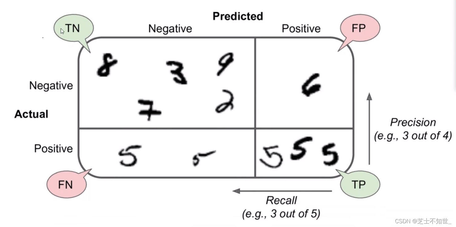
2.2 混淆矩阵Confusion Matrix
分类任务下例对100人进行男女二分类100中模型检测有50人为男(实际全为男)50人为女(实际20为女 30为男)。
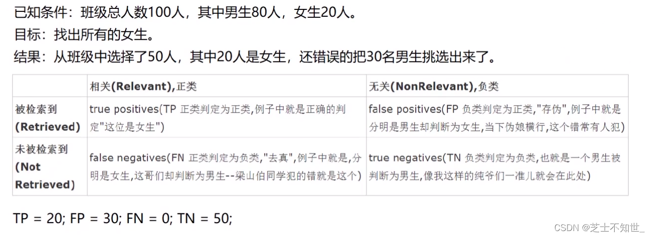
一个完美的分类是只有主对角线非0其他都是0
n分类混淆矩阵就是nxn

接上个代码
from sklearn.model_selection import cross_val_predict
# 60000个数据进行5折交叉验证
# cross_val_predict返回每折预测的结果的concat每折12000个结果5折共60000个结果
y_train_pred = cross_val_predict(sgd_clf, X_train, y_train_5, cv=kfold)
# 画混淆矩阵
from sklearn.metrics import confusion_matrix
confusion=confusion_matrix(y_train_5, y_train_pred)  # 传入train的标签和预测值
# 2分类的矩阵就是2x2的[[TN,FP],[FN,TP]]

plt.figure(figsize=(2, 2))  # 设置图片大小
# 1.热度图后面是指定的颜色块cmap可设置其他的不同颜色
plt.imshow(confusion, cmap=plt.cm.Blues)
plt.colorbar()  # 右边的colorbar
# 2.设置坐标轴显示列表
indices = range(len(confusion))
classes = ['5', 'not 5']
# 第一个是迭代对象表示坐标的显示顺序第二个参数是坐标轴显示列表
plt.xticks(indices, classes, rotation=45)  # 设置横坐标方向rotation=45为45度倾斜
plt.yticks(indices, classes)
# 3.设置全局字体
# 在本例中坐标轴刻度和图例均用新罗马字体['TimesNewRoman']来表示
# ['SimSun']宋体['SimHei']黑体有很多自己都可以设置
plt.rcParams['font.sans-serif'] = ['SimHei']
plt.rcParams['axes.unicode_minus'] = False
# 4.设置坐标轴标题、字体
# plt.ylabel('True label')
# plt.xlabel('Predicted label')
# plt.title('Confusion matrix')
plt.xlabel('预测值')
plt.ylabel('真实值')
plt.title('混淆矩阵', fontsize=12, fontfamily="SimHei")  # 可设置标题大小、字体
# 5.显示数据
normalize = False
fmt = '.2f' if normalize else 'd'
thresh = confusion.max() / 2.
for i in range(len(confusion)):  # 第几行
    for j in range(len(confusion[i])):  # 第几列
        plt.text(j, i, format(confusion[i][j], fmt),
                 fontsize=16,  # 矩阵字体大小
                 horizontalalignment="center",  # 水平居中。
                 verticalalignment="center",  # 垂直居中。
                 color="white" if confusion[i, j] > thresh else "black")
save_flg = True
# 6.保存图片
if save_flg:
    plt.savefig("confusion_matrix.png")
# 7.显示
plt.show()
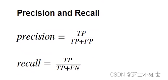
2.3 准确率accuracy、精度precision、召回率recall、F1
sklearn.metrics中有对应的计算函数(y_train, y_train_pred)
准确率accurcy=预测正确个数/总样本数=
T
P
+
T
N
T
P
+
T
N
+
F
P
+
F
N
\frac{TP+TN}{TP+TN+FP+FN}
TP+TN+FP+FNTP+TN
精度precision=
T
P
T
P
+
F
P
\frac{TP}{TP+FP}
TP+FPTP
召回率recall=
T
P
T
P
+
F
N
\frac{TP}{TP+FN}
TP+FNTP
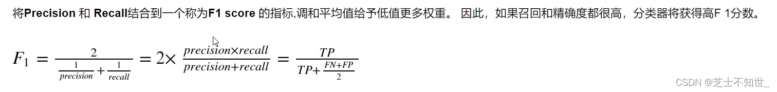
F1 Score=
2
∗
T
P
2
∗
T
P
+
F
P
+
F
N
\frac{2*TP}{2*TP+FP+FN}
2∗TP+FP+FN2∗TP=
2
∗
p
r
e
c
i
s
i
o
n
∗
r
e
c
a
l
l
p
r
e
c
i
s
i
o
n
+
r
e
c
a
l
l
\frac{2*precision*recall}{precision+recall}
precision+recall2∗precision∗recall
接上面代码
from sklearn.metrics import accuracy_score,precision_score,recall_score,f1_score
accuracy=accuracy_score(y_train_5,y_train_pred)
precision=precision_score(y_train_5,y_train_pred)
recall=recall_score(y_train_5,y_train_pred)
f1_score=f1_score(y_train_5,y_train_pred)
print("accuracy=",accuracy)
print("precision=",precision)
print("recall=",recall)
print("f1_score",f1_score)
2.4 置信度confidence
confidence模型对分类预测结果正确的自信程度
y_scores=cross_val_predict(sgd_clf,X_train,y_train_5,kfold,method=‘decision_function’)方法返回每个输入数据的confidence我们可以手动设置阈值t对预测结果进行筛选只有confidence_score>t才视为预测正确。
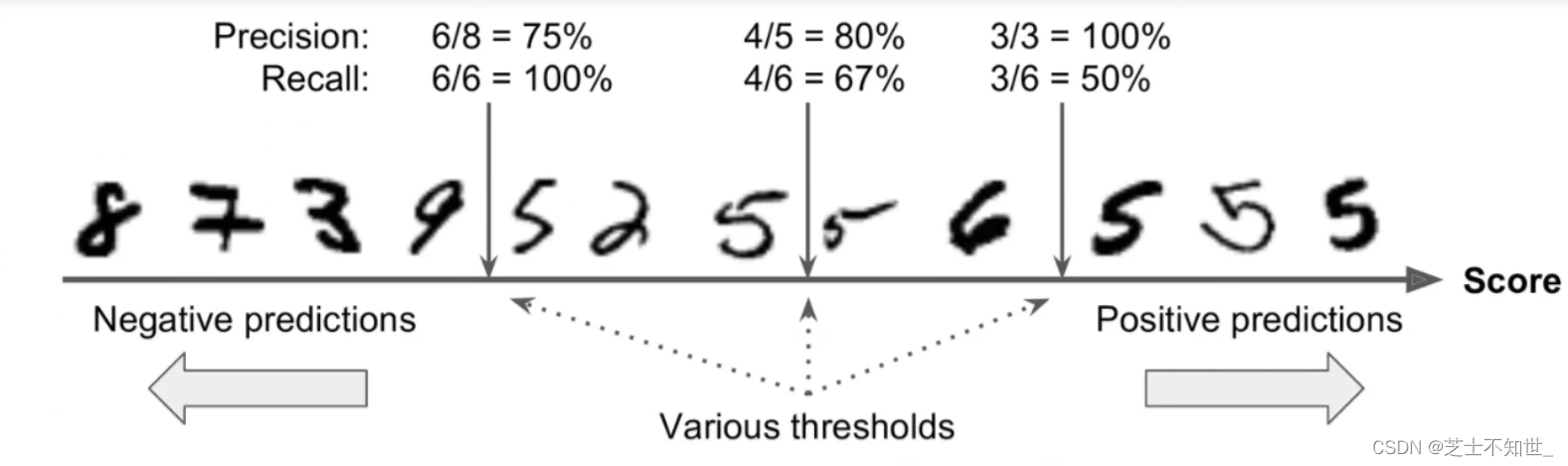
precision, recall, threshholds = precision_recall_curve(y_train_5,y_scores)函数可以自动设置多个阈值且每个阈值都对应计算一遍precision 和 recall

接上面代码
# 自动生成多个阈值并计算precision, recall
y_scores = cross_val_predict(sgd_clf,X_train,y_train_5,kfold,method='decision_function')
from sklearn.metrics import precision_recall_curve
precision, recall, threshholds = precision_recall_curve(y_train_5,y_scores)
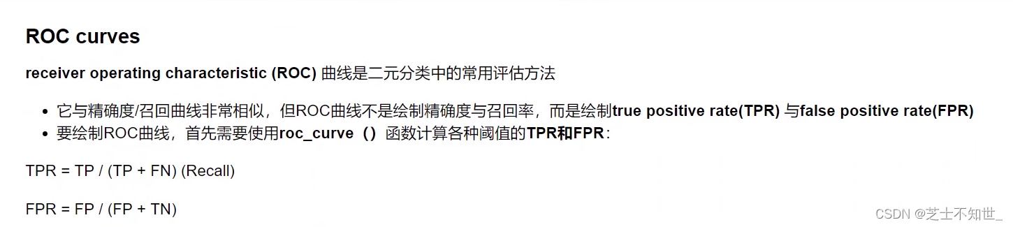
2.5 ROC曲线
分类任务可以画出ROC曲线理想的分类器是逼近左上直角即曲线下方ROC AUC面积接近1.
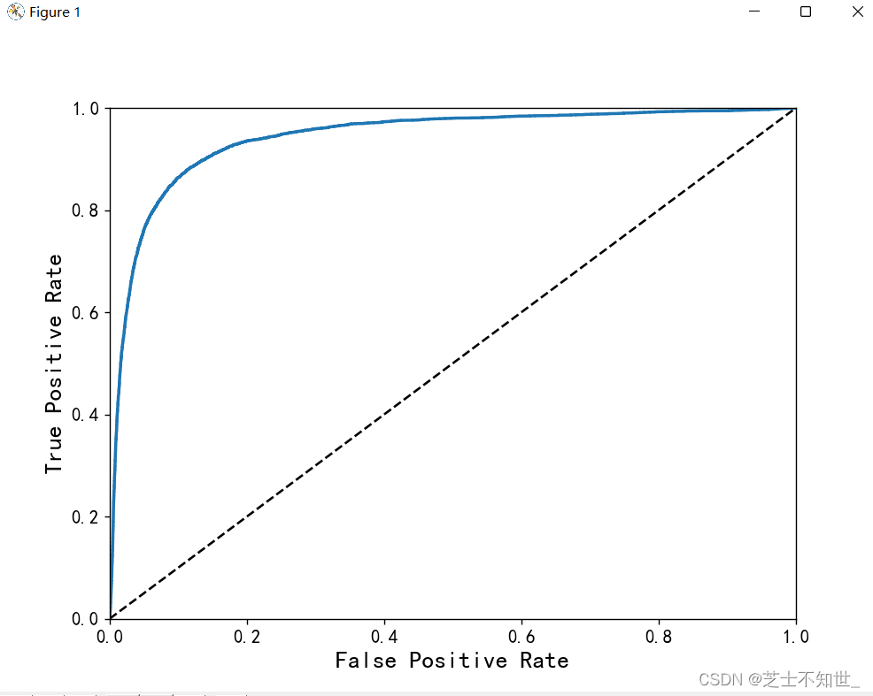
接上面代码
# 分类任务画ROC曲线
from sklearn.metrics import roc_curve
fpr,tpr,threshholds=roc_curve(y_train_5,y_scores)
def plot_roc_curve(fpr,tpr,label=None):
    plt.plot(fpr,tpr,linewidth=2,label=label)
    plt.plot([0,1],[0,1],'k--')
    plt.axis([0,1,0,1])
    plt.xlabel('False Positive Rate', fontsize=16)
    plt.ylabel('True Positive Rate', fontsize=16)
plt.figure(figsize=(8,6))
plot_roc_curve(fpr,tpr)
plt.show()

# 计算roc_auc面积
from sklearn.metrics import roc_auc_score
roc_auc_score=roc_auc_score(y_train_5,y_train_pred)
3.训练调参基本功(LinearRegression)
构建线性回归方程拟合数据点
3.1 线性回归模型实现
准备数据预处理perprocess标准化normalize划分数据集训练集train和测试集test导包sklearn或自己写的class实例化LinearRegression设置超参数lr/eopch/batch…是否制定learning策略学习率衰减策略权重参数初始化init_weight随机初始化/迁移学习训练fit或自己写for迭代计算梯度更新参数预测
3.2不同GD策略对比