CNN 卷积神经网络
| 阿里云国内75折 回扣 微信号:monov8 |
| 阿里云国际,腾讯云国际,低至75折。AWS 93折 免费开户实名账号 代冲值 优惠多多 微信号:monov8 飞机:@monov6 |
文章目录
9、CNN 卷积神经网络
B站视频教程传送门PyTorch深度学习实践 - 卷积神经网络基础篇 PyTorch深度学习实践 - 卷积神经网络高级篇
9.1 Revision
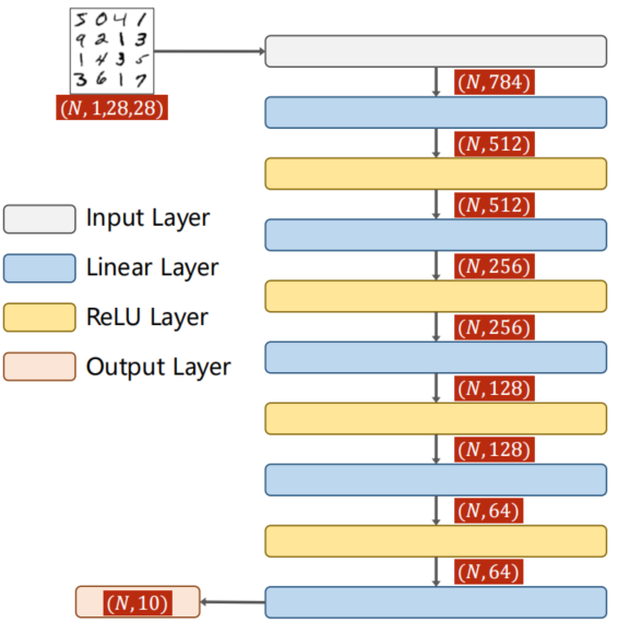
全连接神经网络Fully Connected Neural Network该网络完全由线形层Linear串行连接起来即每一个输入节点都要参与到下一层任一输出节点的计算上。
class Net(torch.nn.Module):
    def __init__(self):
        super(Net, self).__init__()
        self.l1 = torch.nn.Linear(784, 512)
        self.l2 = torch.nn.Linear(512, 256)
        self.l3 = torch.nn.Linear(256, 128)
        self.l4 = torch.nn.Linear(128, 64)
        self.l5 = torch.nn.Linear(64, 10)

    def forward(self, x):
        x = x.view(-1, 784)
        x = F.relu(self.l1(x))
        x = F.relu(self.l2(x))
        x = F.relu(self.l3(x))
        x = F.relu(self.l4(x))
        return self.l5(x)


model = Net()
9.2 Introduction
Convolutional Neural Network

注意
-
1 × 28 × 28 < = = > C × W × H 1 \times 28 \times 28 <==> C \times W \times H 1×28×28<==>C×W×H
-
Convolution 卷积保留图像的空间结构信息
-
Subsampling 下采样主要是 Max Pooling通道数不变宽高改变为了减少图像数据量进一步降低运算的需求
-
Fully Connected 全连接将张量展开为一维向量再进行分类
-
我们将 Convolution 及 Subsampling 等称为特征提取Feature Extraction最后的 Fully Connected 称为分类Classification。
9.3 Convolution

9.3.1 Channel
- Single Input Channel
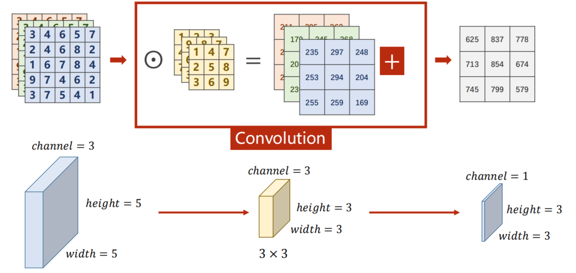
- 3 Input Channels
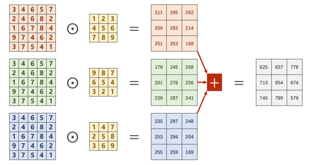
其中C H W 变化如下
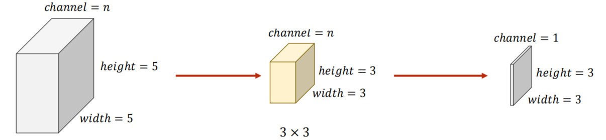
- N Input Channels
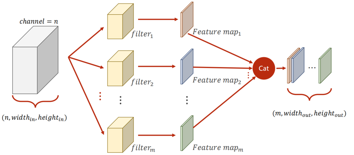
- N Input Channels and M Output Channels
要想输出 M 通道的图像卷积核也需设置为 M 个
9.3.2 Layer
当输入为 n × w i d t h i n × h e i g h t i n n \times width_{in} \times height_{in} n×widthin×heightin 如何得到 m × w i d t h o u t × h e i g h t o u t m \times width_{out} \times height_{out} m×widthout×heightout 的输出

输出的通道数为 m所以需要 m 个卷积核且每个卷积核的尺寸为
n
×
k
e
r
n
e
l
w
i
d
t
h
×
k
e
r
n
e
l
h
e
i
g
h
t
n \times kernel_{width} \times kernel_{height}
n×kernelwidth×kernelheight 即四维张量
m
×
n
×
k
e
r
n
e
l
w
i
d
t
h
×
k
e
r
n
e
l
h
e
i
g
h
t
\Large m \times n \times kernel_{width} \times kernel_{height}
m×n×kernelwidth×kernelheight
import torch

in_channels, out_channels = 5, 10
width, height = 100, 100
kernel_size = 3
batch_size = 1

input = torch.randn(batch_size, in_channels, width, height)
conv_layer = torch.nn.Conv2d(in_channels, out_channels, kernel_size=kernel_size)
output = conv_layer(input)

print(input.shape)
print(conv_layer.weight.shape)  # m n w h
print(output.shape)
torch.Size([1, 5, 100, 100])
torch.Size([10, 5, 3, 3])
torch.Size([1, 10, 98, 98])
9.3.3 Padding
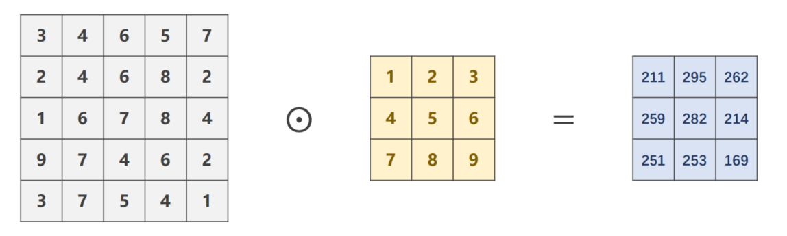
如果 i n p u t = 5 × 5 input = 5 \times 5 input=5×5 k e r n e l = 3 × 3 kernel = 3 \times 3 kernel=3×3 并且希望 o u t p u t = 5 × 5 output = 5 \times 5 output=5×5可以采取什么方法
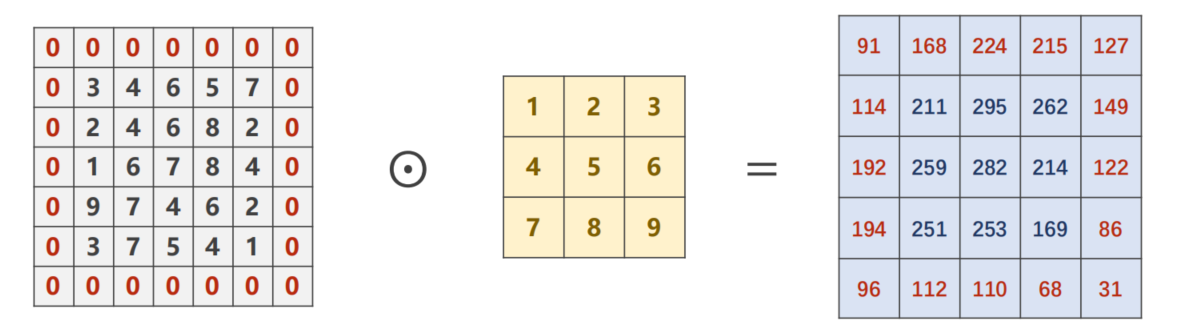
可以使用参数 padding=1 先将input填充至 7 × 7 7 \times 7 7×7 这样卷积之后output仍为 5 × 5 5 \times 5 5×5 。
import torch

input = [3, 4, 6, 5, 7,
         2, 4, 6, 8, 2,
         1, 6, 7, 8, 4,
         9, 7, 4, 6, 2,
         3, 7, 5, 4, 1]

input = torch.Tensor(input).view(1, 1, 5, 5)  # B C W H

conv_layer = torch.nn.Conv2d(in_channels=1, out_channels=1, kernel_size=3, padding=1, bias=False)  # O I W H
kernel = torch.Tensor([1, 2, 3, 4, 5, 6, 7, 8, 9]).view(1, 1, 3, 3)
conv_layer.weight.data = kernel.data

output = conv_layer(input)

print(output)
tensor([[[[ 91., 168., 224., 215., 127.],
          [114., 211., 295., 262., 149.],
          [192., 259., 282., 214., 122.],
          [194., 251., 253., 169.,  86.],
          [ 96., 112., 110.,  68.,  31.]]]], grad_fn=<ConvolutionBackward0>)
9.3.4 Stride
参数 stride 意为步长假设 s t r i d e = 2 stride = 2 stride=2 时kernel在向右或向下移动时一次性移动两格可以有效的降低图像的宽度和高度。
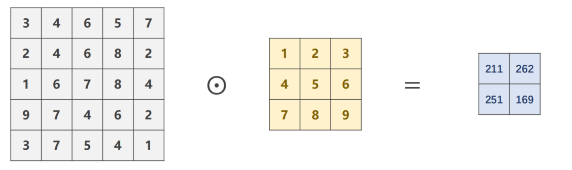
import torch

input = [3, 4, 6, 5, 7,
         2, 4, 6, 8, 2,
         1, 6, 7, 8, 4,
         9, 7, 4, 6, 2,
         3, 7, 5, 4, 1]

input = torch.Tensor(input).view(1, 1, 5, 5)  # B C W H

conv_layer = torch.nn.Conv2d(in_channels=1, out_channels=1, kernel_size=3, stride=2, bias=False)  # O I W H
kernel = torch.Tensor([1, 2, 3, 4, 5, 6, 7, 8, 9]).view(1, 1, 3, 3)
conv_layer.weight.data = kernel.data

output = conv_layer(input)

print(output)
tensor([[[[211., 262.],
          [251., 169.]]]], grad_fn=<ConvolutionBackward0>)
9.4 Max Pooling
Max Pooling最大池化默认 s t r i d e = 2 stride = 2 stride=2 若 k e r n e l = 2 × 2 kernel = 2 \times 2 kernel=2×2 即在该表格中找出最大值

import torch

input = [3, 4, 6, 5,
         2, 4, 6, 8,
         1, 6, 7, 8,
         9, 7, 4, 6]

input = torch.Tensor(input).view(1, 1, 4, 4)
maxpooling_layer = torch.nn.MaxPool2d(kernel_size=2)
output = maxpooling_layer(input)

print(output)
tensor([[[[4., 8.],
          [9., 8.]]]])
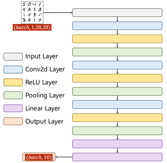
9.5 A Simple CNN
下图为一个简单的神经网络

即

代码如下
class Net(torch.nn.Module):
    def __init__(self):
        super(Net, self).__init__()
        self.conv1 = torch.nn.Conv2d(1, 10, kernel_size=5)
        self.conv2 = torch.nn.Conv2d(10, 20, kernel_size=5)
        self.pooling = torch.nn.MaxPool2d(2)
        self.fc = torch.nn.Linear(320, 10)

    def forward(self, x):
        # Flatten data from (n, 1, 28, 28) to (n, 784)
        batch_size = x.size(0)
        x = F.relu(self.pooling(self.conv1(x)))
        x = F.relu(self.pooling(self.conv2(x)))
        x = x.view(batch_size, -1)  # flatten
        x = self.fc(x)
        return x


model = Net()
9.5.1 GPU
使用GPU来跑数据的前提安装CUDA版PyTorch
- Move Model to GPU 在调用模型后添加以下代码
device = torch.device("cuda:0" if torch.cuda.is_available() else "cpu")
model.to(device)
- Move Tensors to GPU 训练和测试函数添加以下代码
inputs, target = inputs.to(device), target.to(device)
9.5.2 Code 1
import torch
from torchvision import transforms
from torch.utils.data import DataLoader
from torchvision import datasets
import torch.nn.functional as F
import torch.optim as optim
import matplotlib.pyplot as plt
batch_size = 64
transform = transforms.Compose([
transforms.ToTensor(),
transforms.Normalize((0.1307,), (0.3081,))
])
train_dataset = datasets.MNIST(root='../data/mnist', train=True, download=True, transform=transform)
train_loader = DataLoader(train_dataset, shuffle=True, batch_size=batch_size)
test_dataset = datasets.MNIST(root='../data/mnist', train=False, download=True, transform=transform)
test_loader = DataLoader(test_dataset, shuffle=False, batch_size=batch_size)
class Net(torch.nn.Module):
def __init__(self):
super(Net, self).__init__()
self.conv1 = torch.nn.Conv2d(1, 10, kernel_size=5)
self.conv2 = torch.nn.Conv2d(10, 20, kernel_size=5)
self.pooling = torch.nn.MaxPool2d(2)
self.fc = torch.nn.Linear(320, 10)
def forward(self, x):
# Flatten data from (n, 1, 28, 28) to (n, 784)
batch_size = x.size(0)
x = F.relu(self.pooling(self.conv1(x)))
x = F.relu(self.pooling(self.conv2(x)))
x = x.view(batch_size, -1) # flatten
x = self.fc(x)
return x
model = Net()
device = torch.device("cuda:0" if torch.cuda.is_available() else "cpu") # GPU
model.to(device)
criterion = torch.nn.CrossEntropyLoss()
optimizer = optim.SGD(model.parameters(), lr=0.01, momentum=0.5)
def train(epoch):
running_loss = 0.0
for batch_idx, data in enumerate(train_loader, 0):
inputs, target = data
inputs, target = inputs.to(device), target.to(device) # GPU
optimizer.zero_grad()
# forward + backward + update
outputs = model(inputs)
loss = criterion(outputs, target)
loss.backward()
optimizer.step()
running_loss += loss.item()
if batch_idx % 300 == 299:
print('[%d, %3d] loss: %.3f' % (epoch + 1, batch_idx + 1, running_loss / 2000))
running_loss = 0.0
accuracy = []
def test():
correct = 0
total = 0
with torch.no_grad():
for data in test_loader:
inputs, target = data
inputs, target = inputs.to(device), target.to(device) # GPU
outputs = model(inputs)
_, predicted = torch.max(outputs.data, dim=1)
total += target.size(0)
correct += (predicted == target).sum().item()
print('Accuracy on test set: %d %% [%d/%d]' % (100 * correct / total, correct, total))
accuracy.append(100 * correct / total)
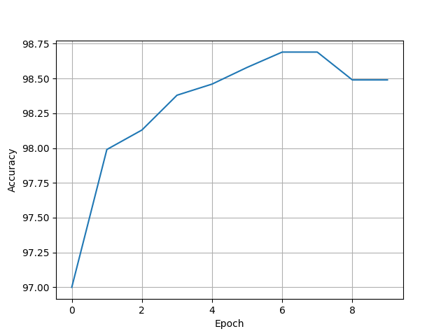
if __name__ == '__main__':
for epoch in range(10):
train(epoch)
test()
print(accuracy)
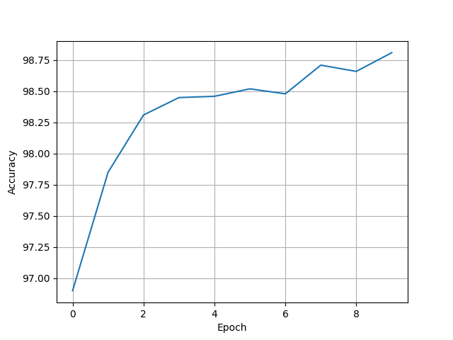
plt.plot(range(10), accuracy)
plt.xlabel("Epoch")
plt.ylabel("Accuracy")
plt.grid()
plt.show()
[1, 300] loss: 0.091
[1, 600] loss: 0.027
[1, 900] loss: 0.020
Accuracy on test set: 97 % [9700/10000]
[2, 300] loss: 0.017
[2, 600] loss: 0.014
[2, 900] loss: 0.013
Accuracy on test set: 97 % [9799/10000]
[3, 300] loss: 0.012
[3, 600] loss: 0.011
[3, 900] loss: 0.011
Accuracy on test set: 98 % [9813/10000]
[4, 300] loss: 0.010
[4, 600] loss: 0.009
[4, 900] loss: 0.009
Accuracy on test set: 98 % [9838/10000]
[5, 300] loss: 0.008
[5, 600] loss: 0.008
[5, 900] loss: 0.008
Accuracy on test set: 98 % [9846/10000]
[6, 300] loss: 0.007
[6, 600] loss: 0.008
[6, 900] loss: 0.007
Accuracy on test set: 98 % [9858/10000]
[7, 300] loss: 0.006
[7, 600] loss: 0.007
[7, 900] loss: 0.007
Accuracy on test set: 98 % [9869/10000]
[8, 300] loss: 0.006
[8, 600] loss: 0.006
[8, 900] loss: 0.006
Accuracy on test set: 98 % [9869/10000]
[9, 300] loss: 0.006
[9, 600] loss: 0.006
[9, 900] loss: 0.006
Accuracy on test set: 98 % [9849/10000]
[10, 300] loss: 0.005
[10, 600] loss: 0.005
[10, 900] loss: 0.005
Accuracy on test set: 98 % [9849/10000]
[97.0, 97.99, 98.13, 98.38, 98.46, 98.58, 98.69, 98.69, 98.49, 98.49]
9.5.3 Exercise
若对该神经网络进行改进
- Conv2d Layer * 3
- ReLU Layer * 3
- MaxPooling Layer * 3
- Linear Layer * 3
i n p u t : 1 × 28 × 28 c o n v o l u t i o n : 28 − 5 + 1 = 24 , t o : 16 × 24 × 24 p o o l i n g : 16 × 12 × 12 c o n v o l u t i o n : 12 − 5 + 1 = 8 , t o : 32 × 8 × 8 p o o l i n g : 20 × 4 × 4 c o n v o l u t i o n : 4 − 3 + 1 = 2 , t o : 64 × 2 × 2 p o o l i n g : 64 × 1 × 1 f c : 64 − − 32 − − 16 − − 10 input: 1 \times 28 \times 28 \\ convolution: 28 -5 +1 = 24, to: 16 \times 24 \times 24 \\ pooling: 16 \times 12 \times 12 \\ convolution: 12 -5 +1 = 8, to: 32 \times 8 \times 8 \\ pooling: 20 \times 4 \times 4 \\ convolution: 4 -3 +1 = 2, to: 64 \times 2 \times 2 \\ pooling: 64 \times 1 \times 1 \\ fc: 64 -- 32 -- 16 -- 10 input:1×28×28convolution:28−5+1=24,to:16×24×24pooling:16×12×12convolution:12−5+1=8,to:32×8×8pooling:20×4×4convolution:4−3+1=2,to:64×2×2pooling:64×1×1fc:64−−32−−16−−10
9.5.4 Code 2
将神经网络改成如下即可
    def __init__(self):
        super(Net, self).__init__()
        self.conv1 = torch.nn.Conv2d(1, 16, kernel_size=5)
        self.conv2 = torch.nn.Conv2d(16, 32, kernel_size=5)
        self.conv3 = torch.nn.Conv2d(32, 64, kernel_size=3)
        self.pooling = torch.nn.MaxPool2d(2)
        self.fc1 = torch.nn.Linear(64, 32)
        self.fc2 = torch.nn.Linear(32, 16)
        self.fc3 = torch.nn.Linear(16, 10)

    def forward(self, x):
        batch_size = x.size(0)
        x = self.pooling(F.relu(self.conv1(x)))
        x = self.pooling(F.relu(self.conv2(x)))
        x = self.pooling(F.relu(self.conv3(x)))
        x = x.view(batch_size, -1)
        x = F.relu(self.fc1(x))
        x = F.relu(self.fc2(x))
        x = self.fc3(x)
        return x
[1, 300] loss: 0.345
[1, 600] loss: 0.273
[1, 900] loss: 0.069
Accuracy on test set: 91 % [9194/10000]
[2, 300] loss: 0.034
[2, 600] loss: 0.025
[2, 900] loss: 0.020
Accuracy on test set: 96 % [9670/10000]
[3, 300] loss: 0.015
[3, 600] loss: 0.015
[3, 900] loss: 0.014
Accuracy on test set: 97 % [9754/10000]
[4, 300] loss: 0.011
[4, 600] loss: 0.010
[4, 900] loss: 0.011
Accuracy on test set: 98 % [9810/10000]
[5, 300] loss: 0.008
[5, 600] loss: 0.009
[5, 900] loss: 0.009
Accuracy on test set: 98 % [9808/10000]
[6, 300] loss: 0.008
[6, 600] loss: 0.007
[6, 900] loss: 0.008
Accuracy on test set: 98 % [9859/10000]
[7, 300] loss: 0.006
[7, 600] loss: 0.006
[7, 900] loss: 0.007
Accuracy on test set: 98 % [9862/10000]
[8, 300] loss: 0.005
[8, 600] loss: 0.006
[8, 900] loss: 0.006
Accuracy on test set: 97 % [9784/10000]
[9, 300] loss: 0.005
[9, 600] loss: 0.005
[9, 900] loss: 0.006
Accuracy on test set: 98 % [9842/10000]
[10, 300] loss: 0.005
[10, 600] loss: 0.005
[10, 900] loss: 0.004
Accuracy on test set: 98 % [9878/10000]
[91.94, 96.7, 97.54, 98.1, 98.08, 98.59, 98.62, 97.84, 98.42, 98.78]

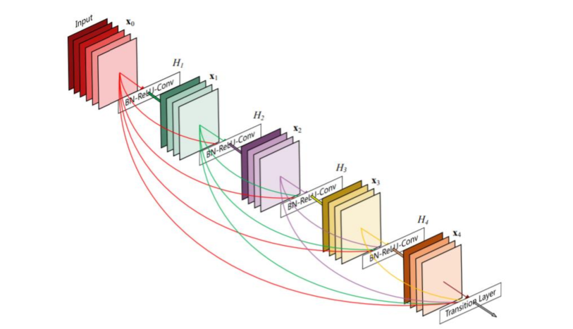
9.6 GoogLeNet
注意Convolution 、 Pooling 、 Softmax、 Other
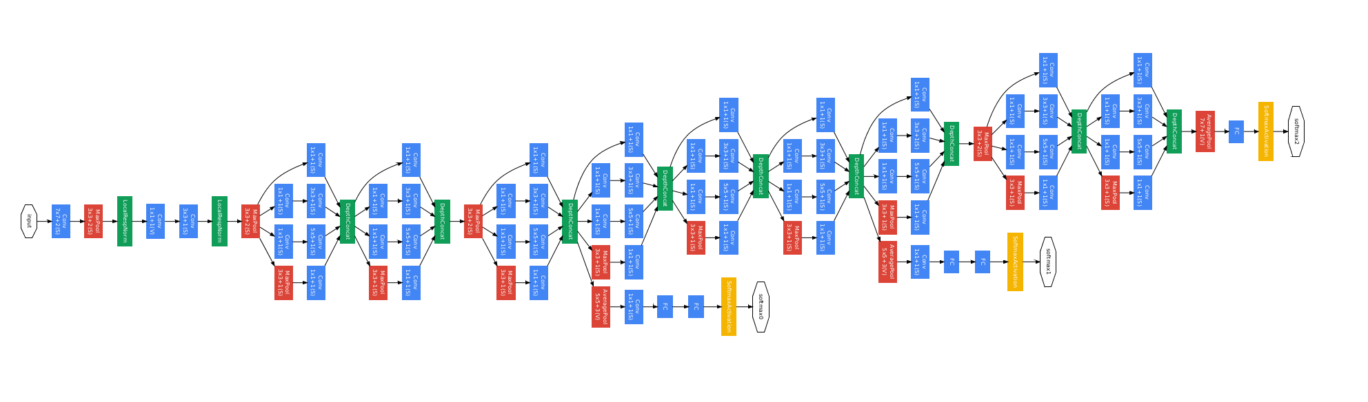
若以上图来编写神经网络则会有许多重复为减少代码冗余可以尽量多使用函数/类。
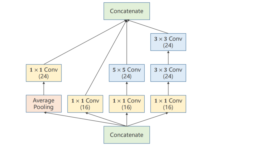
9.6.1 Inception Module
构造神经网络时有一些超参数是难以选择的比如卷积核Kernel应该选择哪一种卷积核比较好用
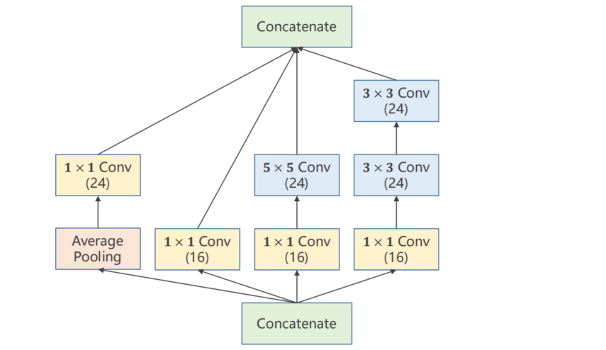
GoogLeNet在一个块中将几种卷积核 1 × 1 、 3 × 3 、 5 × 5 、 . . . 1 \times 1 、 3 \times 3 、 5 \times 5 、... 1×1、3×3、5×5、...都使用然后将其结果罗列到一起将来通过训练自动找到一种最优的组合。
-
Concatenate将张量拼接到一块
-
Average Pooling 均值池化保证输入输出宽高一致可借助padding和stride
9.6.2 1 x 1 convolution
为什么要引入 $1 \times 1 $ convolution
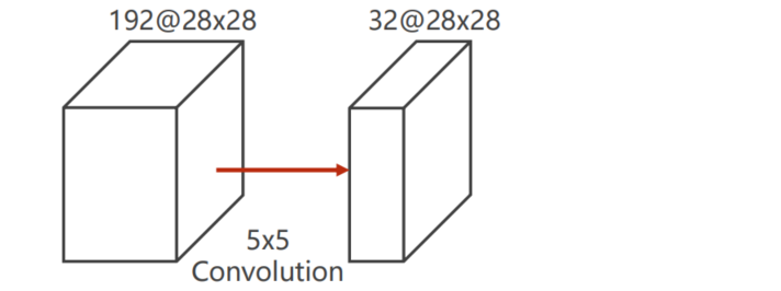
见上图若 i n p u t = 192 × 28 × 28 , o u t p u t = 32 × 28 × 28 input = 192 \times 28 \times 28, output = 32 \times 28 \times 28 input=192×28×28,output=32×28×28 则计算量 O p e r a t i o n s = 5 2 × 2 8 2 × 192 × 32 = 120 , 422 , 400 Operations = 5^2 \times 28^2 \times 192 \times 32 = 120,422,400 Operations=52×282×192×32=120,422,400
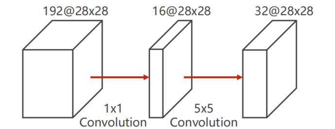
见上图若在其中间使用 c o n v o l u t i o n : 1 × 1 convolution: 1 \times 1 convolution:1×1 则计算量 O p e r a t i o n s = 1 2 × 2 8 2 × 192 × 16 + 5 2 × 2 8 2 × 16 × 32 = 12 , 433 , 648 Operations = 1^2 \times 28^2 \times 192 \times 16 + 5^2 \times 28^2 \times 16 \times 32 = 12,433,648 Operations=12×282×192×16+52×282×16×32=12,433,648
9.6.3 Implementation of Inception Module
计算方向由下至上
# 第一列
self.branch_pool = nn.Conv2d(in_channels, 24, kernel_size=1)

branch_pool = F.avg_pool2d(x, kernel_size=3, stride=1, padding=1)
branch_pool = self.branch_pool(branch_pool)

# 第二列
self.branch1x1 = nn.Conv2d(in_channels, 16, kernel_size=1)

branch1x1 = self.branch1x1(x)

# 第三列
self.branch5x5_1 = nn.Conv2d(in_channels,16, kernel_size=1)
self.branch5x5_2 = nn.Conv2d(16, 24, kernel_size=5, padding=2)

branch5x5 = self.branch5x5_1(x)
branch5x5 = self.branch5x5_2(branch5x5)

# 第四列
self.branch3x3_1 = nn.Conv2d(in_channels, 16, kernel_size=1)
self.branch3x3_2 = nn.Conv2d(16, 24, kernel_size=3, padding=1)
self.branch3x3_3 = nn.Conv2d(24, 24, kernel_size=3, padding=1)

branch3x3 = self.branch3x3_1(x)
branch3x3 = self.branch3x3_2(branch3x3)
branch3x3 = self.branch3x3_3(branch3x3)
再进行拼接

outputs = [branch1x1, branch5x5, branch3x3, branch_pool]
return torch.cat(outputs, dim=1)
Using Inception Module
class InceptionA(nn.Module):
    def __init__(self, in_channels):
        super(InceptionA, self).__init__()
        self.branch1x1 = nn.Conv2d(in_channels, 16, kernel_size=1)

        self.branch5x5_1 = nn.Conv2d(in_channels, 16, kernel_size=1)
        self.branch5x5_2 = nn.Conv2d(16, 24, kernel_size=5, padding=2)

        self.branch3x3_1 = nn.Conv2d(in_channels, 16, kernel_size=1)
        self.branch3x3_2 = nn.Conv2d(16, 24, kernel_size=3, padding=1)
        self.branch3x3_3 = nn.Conv2d(24, 24, kernel_size=3, padding=1)

        self.branch_pool = nn.Conv2d(in_channels, 24, kernel_size=1)

    def forward(self, x):
        branch1x1 = self.branch1x1(x)

        branch5x5 = self.branch5x5_1(x)
        branch5x5 = self.branch5x5_2(branch5x5)

        branch3x3 = self.branch3x3_1(x)
        branch3x3 = self.branch3x3_2(branch3x3)
        branch3x3 = self.branch3x3_3(branch3x3)

        branch_pool = F.avg_pool2d(x, kernel_size=3, stride=1, padding=1)
        branch_pool = self.branch_pool(branch_pool)

        outputs = [branch1x1, branch5x5, branch3x3, branch_pool]
        return torch.cat(outputs, dim=1)
class Net(nn.Module):
    def __init__(self):
        super(Net, self).__init__()
        self.conv1 = nn.Conv2d(1, 10, kernel_size=5)
        self.conv2 = nn.Conv2d(88, 20, kernel_size=5)

        self.incep1 = InceptionA(in_channels=10)
        self.incep2 = InceptionA(in_channels=20)

        self.mp = nn.MaxPool2d(2)
        self.fc = nn.Linear(1408, 10)

    def forward(self, x):
        in_size = x.size(0)
        x = F.relu(self.mp(self.conv1(x)))
        x = self.incep1(x)
        x = F.relu(self.mp(self.conv2(x)))
        x = self.incep2(x)
        x = x.view(in_size, -1)
        x = self.fc(x)
        return x
完整代码
import torch
from torch import nn
from torchvision import transforms
from torchvision import datasets
from torch.utils.data import DataLoader
import torch.nn.functional as F
import torch.optim as optim
import matplotlib.pyplot as plt

# 1、准备数据集
batch_size = 64

transform = transforms.Compose([
    transforms.ToTensor(),
    transforms.Normalize((0.1307,), (0.3081,))
])

train_dataset = datasets.MNIST(root='../data/mnist', train=True, download=True, transform=transform)
train_loader = DataLoader(train_dataset, shuffle=True, batch_size=batch_size)

test_dataset = datasets.MNIST(root='../data/mnist', train=False, download=True, transform=transform)
test_loader = DataLoader(test_dataset, shuffle=False, batch_size=batch_size)


# 2、建立模型
# 定义一个Inception类
class InceptionA(nn.Module):
    def __init__(self, in_channels):
        super(InceptionA, self).__init__()
        self.branch1X1 = nn.Conv2d(in_channels, 16, kernel_size=1)

        # 设置padding保证 宽 高 不变
        self.branch5X5_1 = nn.Conv2d(in_channels, 16, kernel_size=1)
        self.branch5X5_2 = nn.Conv2d(16, 24, kernel_size=5, padding=2)

        self.branch3X3_1 = nn.Conv2d(in_channels, 16, kernel_size=1)
        self.branch3X3_2 = nn.Conv2d(16, 24, kernel_size=3, padding=1)
        self.branch3X3_3 = nn.Conv2d(24, 24, kernel_size=3, padding=1)

        self.branch_pool = nn.Conv2d(in_channels, 24, kernel_size=1)

    def forward(self, x):
        branch1X1 = self.branch1X1(x)

        branch5X5 = self.branch5X5_1(x)
        branch5X5 = self.branch5X5_2(branch5X5)

        branch3X3 = self.branch3X3_1(x)
        branch3X3 = self.branch3X3_2(branch3X3)
        branch3X3 = self.branch3X3_3(branch3X3)

        branch_pool = F.avg_pool2d(x, kernel_size=3, stride=1, padding=1)
        branch_pool = self.branch_pool(branch_pool)

        outputs = [branch1X1, branch5X5, branch3X3, branch_pool]
        # b, c, w, hdim=1 以第一个维度channel来拼接
        return torch.cat(outputs, dim=1)


# 定义模型
class Net(nn.Module):
    def __init__(self):
        super(Net, self).__init__()
        self.conv1 = nn.Conv2d(1, 10, kernel_size=5)
        # 88 = 24*3 + 16
        self.conv2 = nn.Conv2d(88, 20, kernel_size=5)

        self.incep1 = InceptionA(in_channels=10)
        self.incep2 = InceptionA(in_channels=20)

        self.mp = nn.MaxPool2d(2)
        # 确定输出张量的尺寸
        # 在定义时先不定义fc层随便选取一个输入经过模型后查看其尺寸
        # 在init函数中把fc层去掉forward函数中把最后两行去掉确定输出的尺寸后再定义Lear层的大小
        self.fc = nn.Linear(1408, 10)

    def forward(self, x):
        in_size = x.size(0)
        # 1 --> 10
        x = F.relu(self.mp(self.conv1(x)))
        # 10 --> 88
        x = self.incep1(x)
        # 88 --> 20
        x = F.relu(self.mp(self.conv2(x)))
        # 20 --> 88
        x = self.incep2(x)
        x = x.view(in_size, -1)
        x = self.fc(x)
        return x


model = Net()
# 将模型迁移到GPU上运行
device = torch.device("cuda:0" if torch.cuda.is_available() else "cpu")
model.to(device)

# 3、建立损失函数和优化器
criterion = torch.nn.CrossEntropyLoss()
optimizer = optim.SGD(model.parameters(), lr=0.01, momentum=0.5)


# 4、定义训练函数
def train(epoch):
    running_loss = 0
    for batch_idx, data in enumerate(train_loader, 0):
        inputs, target = data

        # 将计算的张量迁移到GPU上
        inputs, target = inputs.to(device), target.to(device)

        optimizer.zero_grad()

        # 前馈 反馈 更新
        outputs = model(inputs)
        loss = criterion(outputs, target)
        loss.backward()
        optimizer.step()

        running_loss += loss.item()
        if batch_idx % 300 == 299:
            print('[%d, %3d] loss: %.3f' % (epoch + 1, batch_idx + 1, running_loss / 300))
            running_loss = 0


# 5、定义测试函数
accuracy = []


def test():
    correct = 0
    total = 0
    with torch.no_grad():
        for data in test_loader:
            images, labels = data

            # 将测试中的张量迁移到GPU上
            images, labels = images.to(device), labels.to(device)

            outputs = model(images)
            _, predicted = torch.max(outputs.data, dim=1)
            total += labels.size(0)
            # 得出其中相等元素的个数
            correct += (predicted == labels).sum().item()
    print('Accuracy on test set: %d %% [%d/%d]' % (100 * correct / total, correct, total))
    accuracy.append(100 * correct / total)


if __name__ == '__main__':
    for epoch in range(10):
        train(epoch)
        test()
    print(accuracy)
    plt.plot(range(10), accuracy)
    plt.xlabel("Epoch")
    plt.ylabel("Accuracy")
    plt.grid()  # 表格
    plt.show()
[1, 300] loss: 0.836
[1, 600] loss: 0.196
[1, 900] loss: 0.145
Accuracy on test set: 96 % [9690/10000]
[2, 300] loss: 0.106
[2, 600] loss: 0.099
[2, 900] loss: 0.091
Accuracy on test set: 97 % [9785/10000]
[3, 300] loss: 0.075
[3, 600] loss: 0.078
[3, 900] loss: 0.071
Accuracy on test set: 98 % [9831/10000]
[4, 300] loss: 0.064
[4, 600] loss: 0.067
[4, 900] loss: 0.061
Accuracy on test set: 98 % [9845/10000]
[5, 300] loss: 0.057
[5, 600] loss: 0.058
[5, 900] loss: 0.052
Accuracy on test set: 98 % [9846/10000]
[6, 300] loss: 0.051
[6, 600] loss: 0.049
[6, 900] loss: 0.050
Accuracy on test set: 98 % [9852/10000]
[7, 300] loss: 0.047
[7, 600] loss: 0.043
[7, 900] loss: 0.045
Accuracy on test set: 98 % [9848/10000]
[8, 300] loss: 0.039
[8, 600] loss: 0.044
[8, 900] loss: 0.042
Accuracy on test set: 98 % [9871/10000]
[9, 300] loss: 0.041
[9, 600] loss: 0.034
[9, 900] loss: 0.041
Accuracy on test set: 98 % [9866/10000]
[10, 300] loss: 0.032
[10, 600] loss: 0.038
[10, 900] loss: 0.037
Accuracy on test set: 98 % [9881/10000]
[96.9, 97.85, 98.31, 98.45, 98.46, 98.52, 98.48, 98.71, 98.66, 98.81]
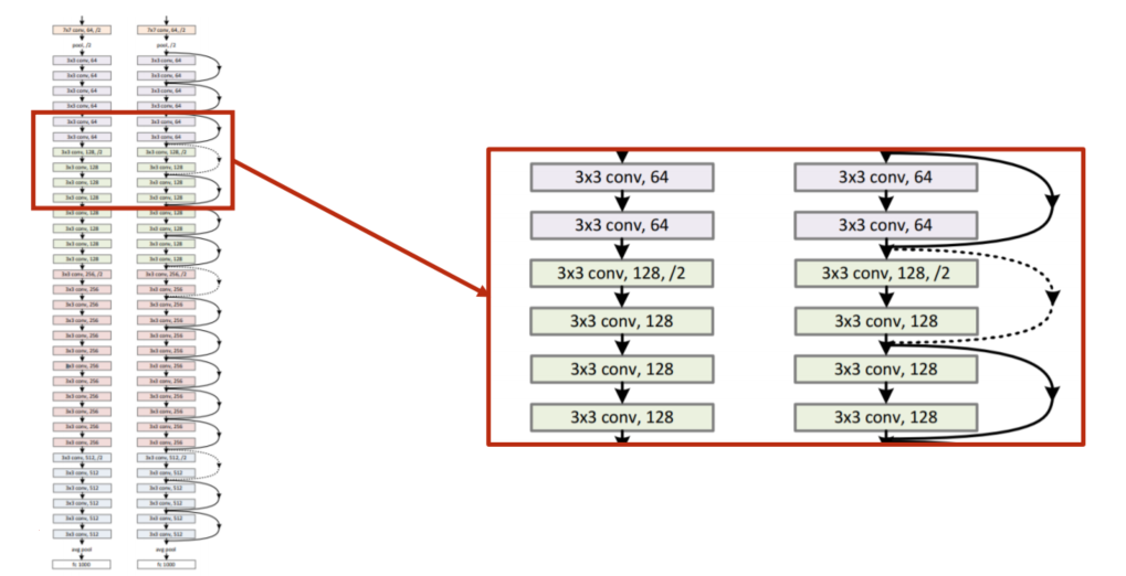
9.7 Residual Net
如果将 3 × 3 3 \times 3 3×3 的卷积一直堆下去该神经网络的性能会不会更好
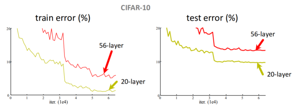
PaperHe K, Zhang X, Ren S, et al. Deep Residual Learning for Image Recognition[C]// IEEE Conference on Computer Vision and Pattern Recognition. IEEE Computer Society, 2016:770-778.
研究发现20 层的错误率低于56 层的错误率所以并不是层数越多性能越好。为解决 梯度消失 的问题见下图
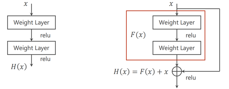
多一个 跳连接
9.7.1 Residual Network

class Net(nn.Module):
    def __init__(self):
        super(Net, self).__init__()
        self.conv1 = nn.Conv2d(1, 16, kernel_size=5)
        self.conv2 = nn.Conv2d(16, 32, kernel_size=5)
        self.mp = nn.MaxPool2d(2)
        self.rblock1 = ResidualBlock(16)
        self.rblock2 = ResidualBlock(32)
        self.fc = nn.Linear(512, 10)

    def forward(self, x):
        in_size = x.size(0)
        x = self.mp(F.relu(self.conv1(x)))
        x = self.rblock1(x)
        x = self.mp(F.relu(self.conv2(x)))
        x = self.rblock2(x)
        x = x.view(in_size, -1)
        x = self.fc(x)
        return x
9.7.2 Residual Block

class ResidualBlock(nn.Module):
    def __init__(self, channels):
        super(ResidualBlock, self).__init__()
        self.channels = channels
        self.conv1 = nn.Conv2d(channels, channels, kernel_size=3, padding=1)
        self.conv2 = nn.Conv2d(channels, channels, kernel_size=3, padding=1)

    def forward(self, x):
        y = F.relu(self.conv1(x))
        y = self.conv2(y)
        return F.relu(x + y)
9.7.3 Code 3
import torch
from torch import nn
from torchvision import transforms
from torchvision import datasets
from torch.utils.data import DataLoader
import torch.nn.functional as F
import torch.optim as optim
import matplotlib.pyplot as plt

batch_size = 64

transform = transforms.Compose([
    transforms.ToTensor(),
    transforms.Normalize((0.1307,), (0.3081,))
])

train_dataset = datasets.MNIST(root='../data/mnist', train=True, download=True, transform=transform)
train_loader = DataLoader(train_dataset, shuffle=True, batch_size=batch_size)

test_dataset = datasets.MNIST(root='../data/mnist', train=False, download=True, transform=transform)
test_loader = DataLoader(test_dataset, shuffle=False, batch_size=batch_size)


class ResidualBlock(nn.Module):
    def __init__(self, channels):
        super(ResidualBlock, self).__init__()
        self.channels = channels
        self.conv1 = nn.Conv2d(channels, channels, kernel_size=3, padding=1)
        self.conv2 = nn.Conv2d(channels, channels, kernel_size=3, padding=1)

    def forward(self, x):
        y = F.relu(self.conv1(x))
        y = self.conv2(y)
        return F.relu(x + y)


class Net(nn.Module):
    def __init__(self):
        super(Net, self).__init__()
        self.conv1 = nn.Conv2d(1, 16, kernel_size=5)
        self.conv2 = nn.Conv2d(16, 32, kernel_size=5)
        self.mp = nn.MaxPool2d(2)

        self.rblock1 = ResidualBlock(16)
        self.rblock2 = ResidualBlock(32)

        self.fc = nn.Linear(512, 10)

    def forward(self, x):
        in_size = x.size(0)
        x = self.mp(F.relu(self.conv1(x)))
        x = self.rblock1(x)
        x = self.mp(F.relu(self.conv2(x)))
        x = self.rblock2(x)
        x = x.view(in_size, -1)
        x = self.fc(x)
        return x


model = Net()

device = torch.device("cuda:0" if torch.cuda.is_available() else "cpu")
model.to(device)

criterion = torch.nn.CrossEntropyLoss()
optimizer = optim.SGD(model.parameters(), lr=0.01, momentum=0.5)


def train(epoch):
    running_loss = 0
    for batch_idx, data in enumerate(train_loader, 0):
        inputs, target = data

        inputs, target = inputs.to(device), target.to(device)
        optimizer.zero_grad()

        outputs = model(inputs)
        loss = criterion(outputs, target)
        loss.backward()
        optimizer.step()

        running_loss += loss.item()
        if batch_idx % 300 == 299:
            print('[%d, %3d] loss: %.3f' % (epoch + 1, batch_idx + 1, running_loss / 300))
            running_loss = 0


accuracy = []


def test():
    correct = 0
    total = 0
    with torch.no_grad():
        for data in test_loader:
            images, labels = data

            images, labels = images.to(device), labels.to(device)
            outputs = model(images)
            _, predicted = torch.max(outputs.data, dim=1)
            total += labels.size(0)

            correct += (predicted == labels).sum().item()
    print('Accuracy on test set: %d %% [%d/%d]' % (100 * correct / total, correct, total))
    accuracy.append(100 * correct / total)


if __name__ == '__main__':
    for epoch in range(10):
        train(epoch)
        test()
    print(accuracy)
    plt.plot(range(10), accuracy)
    plt.xlabel("Epoch")
    plt.ylabel("Accuracy")
    plt.grid()
    plt.show()
[1, 300] loss: 0.563
[1, 600] loss: 0.157
[1, 900] loss: 0.111
Accuracy on test set: 97 % [9721/10000]
[2, 300] loss: 0.085
[2, 600] loss: 0.077
[2, 900] loss: 0.081
Accuracy on test set: 98 % [9831/10000]
[3, 300] loss: 0.063
[3, 600] loss: 0.059
[3, 900] loss: 0.053
Accuracy on test set: 98 % [9841/10000]
[4, 300] loss: 0.047
[4, 600] loss: 0.052
[4, 900] loss: 0.042
Accuracy on test set: 98 % [9877/10000]
[5, 300] loss: 0.039
[5, 600] loss: 0.037
[5, 900] loss: 0.041
Accuracy on test set: 98 % [9871/10000]
[6, 300] loss: 0.035
[6, 600] loss: 0.032
[6, 900] loss: 0.035
Accuracy on test set: 98 % [9895/10000]
[7, 300] loss: 0.029
[7, 600] loss: 0.032
[7, 900] loss: 0.029
Accuracy on test set: 98 % [9899/10000]
[8, 300] loss: 0.026
[8, 600] loss: 0.028
[8, 900] loss: 0.025
Accuracy on test set: 98 % [9892/10000]
[9, 300] loss: 0.021
[9, 600] loss: 0.027
[9, 900] loss: 0.024
Accuracy on test set: 98 % [9886/10000]
[10, 300] loss: 0.019
[10, 600] loss: 0.021
[10, 900] loss: 0.023
Accuracy on test set: 99 % [9902/10000]
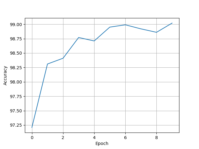
[97.21, 98.31, 98.41, 98.77, 98.71, 98.95, 98.99, 98.92, 98.86, 99.02]
9.7.4 Reading Paper
Paper 1He K, Zhang X, Ren S, et al. Identity Mappings in Deep Residual Networks[C]
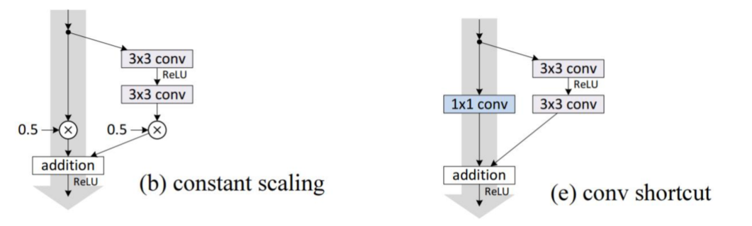
constant scaling
class ResidualBlock(nn.Module):
    def __init__(self, channels):
        super(ResidualBlock, self).__init__()
        self.channels = channels
        self.conv1 = nn.Conv2d(channels, channels, kernel_size=3, padding=1)
        self.conv2 = nn.Conv2d(channels, channels, kernel_size=3, padding=1)

    def forward(self, x):
        y = F.relu(self.conv1(x))
        y = self.conv2(x)
        z = 0.5 * (x + y)
        return F.relu(z)
[1, 300] loss: 1.204
[1, 600] loss: 0.243
[1, 900] loss: 0.165
Accuracy on test set: 96 % [9637/10000]
[2, 300] loss: 0.121
[2, 600] loss: 0.105
[2, 900] loss: 0.099
Accuracy on test set: 97 % [9777/10000]
[3, 300] loss: 0.085
[3, 600] loss: 0.076
[3, 900] loss: 0.069
Accuracy on test set: 98 % [9815/10000]
[4, 300] loss: 0.061
[4, 600] loss: 0.063
[4, 900] loss: 0.063
Accuracy on test set: 98 % [9849/10000]
[5, 300] loss: 0.053
[5, 600] loss: 0.052
[5, 900] loss: 0.052
Accuracy on test set: 98 % [9853/10000]
[6, 300] loss: 0.041
[6, 600] loss: 0.051
[6, 900] loss: 0.047
Accuracy on test set: 98 % [9871/10000]
[7, 300] loss: 0.040
[7, 600] loss: 0.044
[7, 900] loss: 0.043
Accuracy on test set: 98 % [9869/10000]
[8, 300] loss: 0.039
[8, 600] loss: 0.038
[8, 900] loss: 0.037
Accuracy on test set: 98 % [9859/10000]
[9, 300] loss: 0.031
[9, 600] loss: 0.039
[9, 900] loss: 0.036
Accuracy on test set: 98 % [9875/10000]
[10, 300] loss: 0.035
[10, 600] loss: 0.031
[10, 900] loss: 0.033
Accuracy on test set: 98 % [9888/10000]
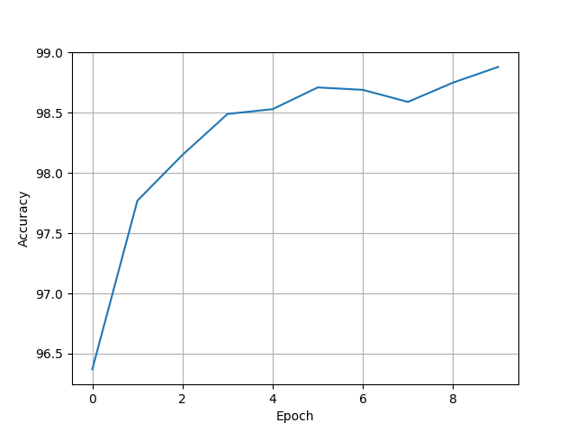
[96.37, 97.77, 98.15, 98.49, 98.53, 98.71, 98.69, 98.59, 98.75, 98.88]
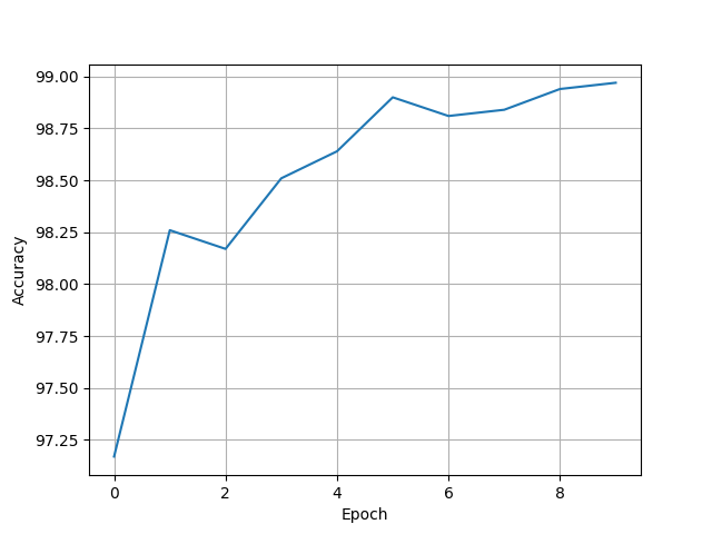
conv shortcut
class ResidualBlock(nn.Module):
    def __init__(self, channels):
        super(ResidualBlock, self).__init__()
        self.channels = channels

        self.conv1 = nn.Conv2d(channels, channels, kernel_size=3, padding=1)
        self.conv2 = nn.Conv2d(channels, channels, kernel_size=3, padding=1)
        self.conv3 = nn.Conv2d(channels, channels, kernel_size=1)

    def forward(self, x):
        y = F.relu(self.conv1(x))
        y = self.conv2(x)
        z = self.conv3(x) + y
        return F.relu(z)
[1, 300] loss: 0.760
[1, 600] loss: 0.170
[1, 900] loss: 0.119
Accuracy on test set: 97 % [9717/10000]
[2, 300] loss: 0.092
[2, 600] loss: 0.084
[2, 900] loss: 0.075
Accuracy on test set: 98 % [9826/10000]
[3, 300] loss: 0.064
[3, 600] loss: 0.063
[3, 900] loss: 0.055
Accuracy on test set: 98 % [9817/10000]
[4, 300] loss: 0.048
[4, 600] loss: 0.047
[4, 900] loss: 0.048
Accuracy on test set: 98 % [9851/10000]
[5, 300] loss: 0.039
[5, 600] loss: 0.039
[5, 900] loss: 0.044
Accuracy on test set: 98 % [9864/10000]
[6, 300] loss: 0.035
[6, 600] loss: 0.033
[6, 900] loss: 0.038
Accuracy on test set: 98 % [9890/10000]
[7, 300] loss: 0.030
[7, 600] loss: 0.030
[7, 900] loss: 0.030
Accuracy on test set: 98 % [9881/10000]
[8, 300] loss: 0.027
[8, 600] loss: 0.026
[8, 900] loss: 0.029
Accuracy on test set: 98 % [9884/10000]
[9, 300] loss: 0.021
[9, 600] loss: 0.026
[9, 900] loss: 0.025
Accuracy on test set: 98 % [9894/10000]
[10, 300] loss: 0.019
[10, 600] loss: 0.019
[10, 900] loss: 0.025
Accuracy on test set: 98 % [9897/10000]
[97.17, 98.26, 98.17, 98.51, 98.64, 98.9, 98.81, 98.84, 98.94, 98.97]
Paper 2Huang G, Liu Z, Laurens V D M, et al. Densely Connected Convolutional Networks[J]. 2016:2261-2269.