机器学习笔记之变分自编码器(一)模型表示

引言

本节将介绍变分自编码器(Variational AutoEncoder,VAE)。

回顾：高斯混合模型

高斯混合模型本质上是 $\mathcal{K}$个高斯分布的混合分布。它的概率图结构表示如下：

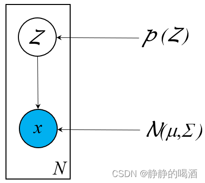
其中$\mathcal{Z}$是一个离散型随机变量一共包含$\mathcal{K}$种选择结果(服从$\text{Categorical}$分布)；并且隐变量$\mathcal{Z}$的每个取值$z_j\in \mathcal{Z}$均唯一对应一个高斯分布$\mathcal{N}({\mu }_j,{\Sigma }_j)$：
并满足${\sum }_{k=1}^{\mathcal{K}}=1$.

$\mathcal{Z}$	$z_1$	$z_2$	$\cdots$	$z_{\mathcal{K}}$
$\mathcal{P}(\mathcal{Z})$	$p_1$	$p_2$	$\cdots$	$p_{\mathcal{K}}$
$\mathcal{P}(x\mid \mathcal{Z})$	$\mathcal{N}({\mu }_1,{\Sigma }_1)$	$\mathcal{N}({\mu }_2,{\Sigma }_2)$	$\cdots$	$\mathcal{N}({\mu }_{\mathcal{K}},{\Sigma }_{\mathcal{K}})$

变分自编码器——概率图视角介绍

从模型名称观察：

• 变分自编码器中的变分自然是指变分推断(Variational Inference,VI)；这个概念来自于概率图模型对变量(隐变量)的条件概率进行求解。
• 变分自编码器中的自编码器(AutoEncoder,AE)来自于前馈神经网络结构。不同于概率图模型它是一种计算图结构；并且它的底层逻辑是通用逼近定理通过各网络层的参数对概率分布进行表达。

因此变分自编码器是一种典型的：

• 概率图、计算图相结合的模型；
• 它也是一个隐变量模型(Latent Variable Model,LVM)。它的概率图结构表示如下：
  
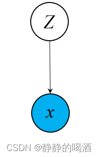
• 它也是一个静态模型(Static Model)。
  这里主要是区别于‘隐马尔可夫模型’系列的动态模型(Dynamic Model)。

在之前的介绍中提到过一种简单的静态隐变量模型——高斯混合模型(Gaussian Mixture Model,GMM)观察高斯混合模型与变分自编码器之间的关联关系。

如果从若干个高斯分布混合的角度观察高斯混合模型那么变分自编码器可看作 无限个高斯分布混合。在高斯混合模型中隐变量$\mathcal{Z}$被假设为$1$维、服从$\text{Categorical}$分布的离散型随机变量。

而高斯混合模型常用于处理无监督的聚类任务。换句话说因为隐变量$\mathcal{Z}$的假设或者说它的复杂程度过于简单使得高斯混合模型只能处理 浅层特征。相反如果给定一张图片去执行图像识别或者是目标检测$\text{GMM}$显然是无法实现的。
如何从探索深层特征？这需要提高隐变量$\mathcal{Z}$的复杂程度：

• (特征维度角度的扩展)$\mathcal{Z}$：$1$维特征 $\Rightarrow$ 高维特征；
  需要注意的是这里的下标表示随机变量的维度下标不同于上面的取值下标,$\mathcal{M}$表示维度数量。
  $$\mathcal{Z}=(z_1,z_2,\cdots ,z_{\mathcal{M}}{)}^T$$
• (随机变量性质角度的扩展)$\mathcal{Z}$：离散型随机变量 $\Rightarrow$ 连续型随机变量。

这里不妨假设$\mathcal{Z}$服从高斯分布：
均值为0,协方差矩阵为标准单位矩阵${\mathcal{I}}_{\mathcal{M}\times \mathcal{M}}$.
$$\mathcal{Z}\sim \mathcal{N}(0,{\mathcal{I}}_{\mathcal{M}\times \mathcal{M}})$$
在给定隐变量$\mathcal{Z}$的条件下样本$x$的后验分布$x\mid \mathcal{Z}$可分为两种情况：
这里仅对$x$是连续型随机变量进行讨论。

• 如果$x$是离散型随机变量那么$x$将服从$\text{Categorical}$分布或者是伯努利分布(视情况而定)；
  这里需要注意的是这个$\text{Categorical}$分布是针对$x$的区别于高斯混合模型中针对$\mathcal{Z}$的分布。
• 如果$x$是连续型随机变量那么通常将$x$服从高斯分布：
  • 注意：这里将高斯分布的期望、协方差$\mu ,\Sigma$描述成关于'给定条件'$\mathcal{Z}$的函数函数对应的权重参数设置为$\theta$.
  • 设置成$\mu (\mathcal{Z};\theta ),\Sigma (\mathcal{Z};\theta )$的目的是使用神经网络的‘通用逼近定理’去近似学习$\theta$,从而得到$\mu ,\Sigma$的近似解。
    $$x\mid \mathcal{Z}\sim \mathcal{N}\left[\mu (\mathcal{Z};\theta ),\Sigma (\mathcal{Z};\theta )\right]$$

之所以使用神经网络来学习权重参数$\theta$表示$\mu (\mathcal{Z};\theta ),\Sigma (\mathcal{Z};\theta )$是因为隐变量$\mathcal{Z}$可能维度/复杂程度极高即便使用重参数化技巧来近似求解分布也是极为复杂的。

• 以随机梯度变分推断为例关于假定分布$\mathcal{Q}(\mathcal{Z})$的变分$\mathcal{L}[\mathcal{Q}(\mathcal{Z})]$可表示为关于参数$\varphi$的函数形式：(这里将假定分布$\mathcal{Q}(\mathcal{Z})$看做一个关于$\varphi$的函数),推导过程详见随机梯度变分推断($\text{SGVI}$)
  这里的$\mathcal{X}$指观测变量(样本)的随机变量集合。
  $$\begin{array}{rl}\mathcal{L}[\mathcal{Q}(\mathcal{Z})]& =\underset{\text{ELBO}}{\underbrace{{\mathbb{E}}_{\mathcal{Q}(\mathcal{Z};\varphi )}\left[\log \mathcal{P}(\mathcal{X},\mathcal{Z})-\log \mathcal{Q}(\mathcal{Z};\varphi )\right]}}=\mathcal{L}(\varphi )\end{array}$$
• 而变分关于$\varphi$的梯度${\nabla }_{\varphi }\mathcal{L}(\varphi )$最终可以表示成期望形式:
  ∇ ϕ L ( ϕ ) = E Q ( Z ; ϕ ) { ∇ ϕ log ⁡ Q ( Z ; ϕ ) ⋅ [ log ⁡ P ( X , Z ) − log ⁡ Q ( Z ; ϕ ) ] } \nabla_{\phi}\mathcal L(\phi) = \mathbb E_{\mathcal Q(\mathcal Z;\phi)} \left\{\nabla_{\phi}\log \mathcal Q(\mathcal Z;\phi) \cdot \left[\log \mathcal P(\mathcal X,\mathcal Z) - \log \mathcal Q(\mathcal Z;\phi)\right]\right\} ∇ϕ​L(ϕ)=EQ(Z;ϕ)​{∇ϕ​logQ(Z;ϕ)⋅[logP(X,Z)−logQ(Z;ϕ)]}
  而在使用‘蒙特卡洛方法’近似过程中首先针对${\nabla }_{\varphi }\mathcal{L}(\varphi )$的近似需要采集大量样本其次也会出现高方差的现象。虽然使用‘重参数化技巧’能够有效减小高方差的现象但本质依然需要大量采样:
  $$\begin{gathered} \mathcal{Z}=\mathcal{G}(ϵ,\mathcal{X};\varphi ) \\ {\nabla }_{\varphi }\mathcal{L}(\varphi )={\mathbb{E}}_{\mathcal{P}(ϵ)}\left[{\nabla }_{\mathcal{Z}}\left[\log \mathcal{P}(\mathcal{X},\mathcal{Z})-\log \mathcal{Q}(\mathcal{Z};\varphi )\right]\cdot {\nabla }_{\varphi }\mathcal{G}(ϵ,\mathcal{X};\varphi )\right] \end{gathered}$$
  如果$\mathcal{Z}$维度足够高那么意味着假定分布$\mathcal{Q}(\mathcal{Z})$足够复杂因而需要采集足够的样本去近似${\nabla }_{\varphi }\mathcal{L}(\varphi )$,这仅是梯度上升的一次迭代计算代价是极高的。

如果使用$x\mid \mathcal{Z}\sim \mathcal{N}\left[\mu (\mathcal{Z};\theta ),\Sigma (\mathcal{Z};\theta )\right]$这种假设那么关于观测变量集合$\mathcal{X}$的边缘概率分布可表示为：

• 其中$\mathcal{P}(\mathcal{Z})$指隐变量$\mathcal{Z}$的先验概率：$\mathcal{Z}\sim \mathcal{N}(0,{\mathcal{I}}_{\mathcal{M}\times \mathcal{M}})$,但在前馈神经网络结构的学习过程中$\mathcal{Z}$的先验分布显得并不重要。和生成对抗网络(GAN)中关于生成模型中的输入一样它就仅是满足“高维、连续”条件的一个简单分布。
• 相比于先验分布$\mathcal{P}(\mathcal{Z})$我们实际上更关心'后验概率'$\mathcal{P}(\mathcal{Z}\mid \mathcal{X})$,即通过样本的学习出的隐变量的分布信息。
  
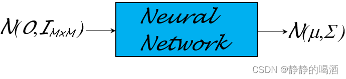
• 但变分自编码器中关于噪声部分的输出是高斯分布这里只是假定$x\mid \mathcal{Z}$服从高斯分布$\mathcal{N}\left[\mu (\mathcal{Z};\theta ),\Sigma (\mathcal{Z};\theta )\right]$但它实际上可能是任意分布。但有神经网络的通用逼近定理不需要担心它仅是使用一个简单高斯分布$\mathcal{N}(0,{\mathcal{I}}_{\mathcal{M}\times \mathcal{M}})$作为输入通过模型参数逼近真实的噪声分布(见图)。

$$\begin{array}{rl}\mathcal{P}(\mathcal{X})& ={\int }_{\mathcal{Z}}\mathcal{P}(\mathcal{X},\mathcal{Z})d\mathcal{Z}\\ & ={\int }_{\mathcal{Z}}\underset{\text{Prior}}{\underbrace{\mathcal{P}(\mathcal{Z})}}\cdot \mathcal{P}(\mathcal{X}\mid \mathcal{Z})d\mathcal{Z}\{\begin{array}{l}\mathcal{Z}\sim \mathcal{N}(0,{\mathcal{I}}_{\mathcal{M}\times \mathcal{M}})\\ \mathcal{X}\mid \mathcal{Z}\sim \mathcal{N}\left[\mu (\mathcal{Z};\theta ),\Sigma (\mathcal{Z};\theta )\right]\end{array}\end{array}$$

如果基于上述假设此时隐变量$\mathcal{Z}$的维度极高($\mathcal{M}$)这导致${\int }_{\mathcal{Z}}$是极复杂的甚至是 无法处理的($\text{Intractable}$)。这导致$\mathcal{P}(\mathcal{X})$也是无法直接求解的：
$$\begin{array}{rl}\underset{\text{Intractable}}{\underbrace{\mathcal{P}(\mathcal{X})}}& ={\int }_{\mathcal{Z}}\left[\mathcal{P}({\mathcal{Z}}_1,\cdots ,{\mathcal{Z}}_{\mathcal{M}})\cdot \mathcal{P}(\mathcal{X}\mid {\mathcal{Z}}_1,\cdots {\mathcal{Z}}_{\mathcal{M}})\right]d{\mathcal{Z}}_1,\cdots {\mathcal{Z}}_{{\mathcal{Z}}_{\mathcal{M}}}\\ & ={\int }_{{\mathcal{Z}}_1}{\int }_{{\mathcal{Z}}_2}\cdots {\int }_{{\mathcal{Z}}_{\mathcal{M}}}\left[\mathcal{P}({\mathcal{Z}}_1,\cdots ,{\mathcal{Z}}_{\mathcal{M}})\cdot \mathcal{P}(\mathcal{X}\mid {\mathcal{Z}}_1,\cdots {\mathcal{Z}}_{\mathcal{M}})\right]d{\mathcal{Z}}_1,\cdots {\mathcal{Z}}_{{\mathcal{Z}}_{\mathcal{M}}}\end{array}$$
根据贝叶斯定理关于隐变量的后验分布$\mathcal{P}(\mathcal{Z}\mid \mathcal{X})$同样是无法处理的($\text{Intractable}$)：
也就是贝叶斯定理自身的‘积分难问题’。
$$\underset{\text{Intractable}}{\underbrace{\mathcal{P}(\mathcal{Z}\mid \mathcal{X})}}=\frac{\mathcal{P}(\mathcal{X},\mathcal{Z})}{\mathcal{P}(\mathcal{X})}=\frac{\mathcal{P}(\mathcal{Z})\cdot \mathcal{P}(\mathcal{X}\mid \mathcal{Z})}{\mathcal{P}(\mathcal{X})}$$

总结

从概率图视角观察变分自编码器就是一个隐变量模型($\text{Latent Variable Model}$)相比于高斯混合模型的建模思路变分自编码器的特点是隐变量$\mathcal{Z}$足够复杂——$\mathcal{Z}$被假设为高维、连续的随机变量。

这里仅将$\mathcal{P}(\mathcal{Z})$设置成一个满足高维、连续的简单分布：
$$\mathcal{Z}\sim \mathcal{N}(0,{\mathcal{I}}_{\mathcal{M}\times \mathcal{M}})$$
因为隐变量$\mathcal{Z}$是建模过程中假设的变量在没有真实样本$\mathcal{X}$的条件下先验分布$\mathcal{P}(\mathcal{Z})$并不重要。在极大似然估计与最大后验概率估计一节中介绍过当真实样本足够多的时候先验概率的权重会逐渐缩减。而生成过程$\mathcal{P}(\mathcal{X}\mid \mathcal{Z})$的概率分布通常设置为如下形式：
$$\mathcal{X}\mid \mathcal{Z}\sim \mathcal{N}\left[\mu (\mathcal{Z};\theta ),\Sigma (\mathcal{Z};\theta )\right]$$
需要注意的是虽然这里写成了高斯分布的格式但实际上它可能是任意噪声分布。由于$\mathcal{Z}$维度可能过于复杂仅通过蒙特卡洛方法采样(随机梯度变分推断($\text{SGVI}$)重参数化技巧等)计算代价极高。因此使用神经网络调整参数$\theta$使$\mathcal{N}\left[\mu (\mathcal{Z};\theta ),\Sigma (\mathcal{Z};\theta )\right]$逼近任意噪声分布。

相比之下我们更关心隐变量的后验分布$\mathcal{P}(\mathcal{Z}\mid \mathcal{X};\theta )$。因为此时的隐变量分布在真实样本的加持下具有了实际意义。但根据贝叶斯定理$\mathcal{P}(\mathcal{Z}\mid \mathcal{X};\theta )$同样存在积分难问题：
这里的$\mathcal{P}(\mathcal{Z})$与对应的$\mathcal{P}({\mathcal{Z}}_1,\cdots {\mathcal{Z}}_{\mathcal{M}})$均指的使先验分布它们作为神经网络的输入并不会更新自身梯度。因此这里没有加$\theta$.
$$\begin{array}{rl}\underset{\text{Intractable}}{\underbrace{\mathcal{P}(\mathcal{Z}\mid \mathcal{X};\theta )}}& =\frac{\mathcal{P}(\mathcal{Z})\cdot \mathcal{P}(\mathcal{X}\mid \mathcal{Z};\theta )}{\underset{\text{Intractable}}{\underbrace{\mathcal{P}(\mathcal{X};\theta )}}}\{\begin{array}{l}\mathcal{Z}\sim \mathcal{N}(0,{\mathcal{I}}_{\mathcal{M}\times \mathcal{M}})\\ \mathcal{X}\mid \mathcal{Z}\sim \mathcal{N}\left[\mu (\mathcal{Z};\theta ),\Sigma (\mathcal{Z};\theta )\right]\end{array}\\ \mathcal{P}(\mathcal{X};\theta )& ={\int }_{{\mathcal{Z}}_1}\cdots {\int }_{{\mathcal{Z}}_{\mathcal{M}}}\left[\mathcal{P}({\mathcal{Z}}_1,\cdots ,{\mathcal{Z}}_{\mathcal{M}})\cdot \mathcal{P}(\mathcal{X}\mid {\mathcal{Z}}_1,\cdots {\mathcal{Z}}_{\mathcal{M}};\theta )\right]d{\mathcal{Z}}_1,\cdots {\mathcal{Z}}_{\mathcal{M}}\end{array}$$

因此需要使用推断的方式将$\mathcal{P}(\mathcal{Z}\mid \mathcal{X})$求解出来从而实现样本的生成过程。

下一节将介绍变分自编码器的推断过程。

相关参考：
变分自编码器——模型表示