【计算几何】德劳内三角剖分算法 | 利用 scatter 绘制散点图 | 实现外接圆生成 | scipy库的 Dealunay 函数 | 实战: A-B间欧氏距离计算_python三维三角剖分

阿里云国内75折回扣微信号：monov8

阿里云国际，腾讯云国际，低至75折。AWS 93折免费开户实名账号代冲值优惠多多微信号：monov8 飞机：@monov6

猛戳跟哥们一起玩蛇啊 👉 《一起玩蛇》🐍

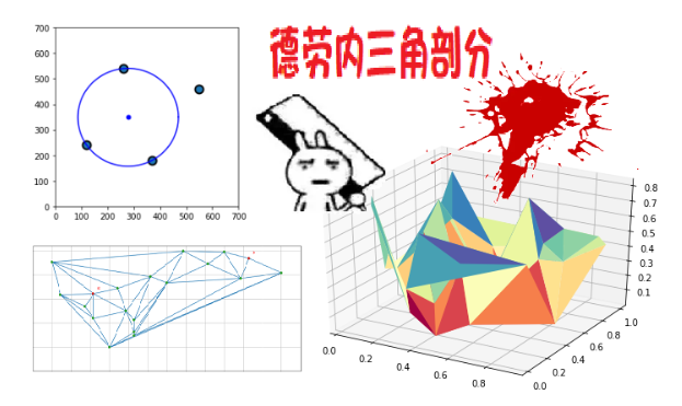
💭 写在前面本章我们将介绍的是计算机和领域的 Delaunay 三角剖分算法即德劳内三角剖分它是一种用于将点集划分成三角形网格的算法。点集的三角剖分属于计算几何学科范畴对数值分析、有限元分析与图形学来说是极为重要的一项预处理技术。得益于德劳内三角剖分的独特性关于点集的很多种几何图都与德劳内三角剖分密切相关如沃罗诺伊图EMST 树Gabriel 图等。本章我们介绍完之后下一章我们就介绍介绍沃罗诺伊图。柠檬叶子C经典表情包写作风格暂时下架本篇博客没有表情包唯一的表情包就是开头放了个兔斯基拿大砍刀的表情。

本篇博客全站热榜排名13

Ⅰ. 前置知识

0x00 引入什么是德劳内三角剖分

当用三角形连接平面上的点来剖分空间时剖分使得这些三角形的内角的最小值变为最大值。

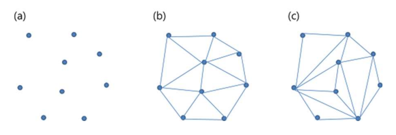
当有 $(a)$ 中的点时通过连接这些点的方法来构成三角形的方式多的 "一笔雕凿"

作为一个南京人我来给大家解释解释这里的一笔雕凿是什么意思。

一笔雕凿指的是用一支笔去雕刻凿出精美的工艺品是传统代笔手艺人的基本功。

多用于表示 "非常、极致" 在句子通常作状语修饰形容词形容程度极深

比如这里使用是对连点构成三角形的 "方法非常多" 的感叹。

而我们所探讨的 —— "徳劳内三角剖分" 则是让每个三角形都尽可能接近 $(b)$ 所示的等边三角形的剖分确保不会出现 $(c)$ 中的那种细长三角形。

德劳内三角剖分需要满足任意一个三角形的外接圆是空圆。

任意的一个三角形的外接圆内部是没有点的每一个三角形的内部都没有点。

德劳内三角剖分使得每个三角形内部的圆心在该三角形内部并且没有其他点在圆内。

三角形越细长外切圆也越大。比如在上图中 $(b)$ 满足此条件 $(c)$ 就不满足。

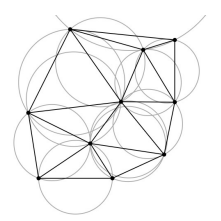显示外接圆的三角剖分

0x01 学会利用 scatter 函数绘制散点图

我们先学习如何生成散点我们一般用 matplotlib 库中的 scatter 函数生成散点图。

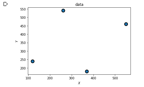
💬 代码演示绘制一个带有四个散点的散点图

# from sklearn.datasets import make_classification
import numpy as np
import matplotlib .pyplot as plt

points = [
    (120,240), (370,180), (550,460), (260,540)  # 定义散点的坐标
]
points = np.array(points) # 输出到图像

plt.title("data")         # 设置图像标题

## 利用 Matplotlib 中的 scatter 函数绘制散点图
plt.scatter (
    points[:, 0],         # 对应散点图中每个点的 x 坐标
    points[:, 1],         # 对于散点图中每个点的 y 坐标
    marker = 'o',         # maker参数指定散点图中每个散点的形状
    s = 100,              # 指定了散点图中每个散点的大小
    edgecolor = "k",      # 指定了散点图中每个散点的边缘颜色。
    linewidth = 2         # 参数指定了散点图中每个散点边缘的线宽。
)

plt.xlabel("$X$")         # 设置x坐标轴标签
plt.ylabel("$Y$")         # 设置y坐标轴标签
plt.show()                # 显示图像

🚩 运行结果

💡 分析

运行代码后成功生成了带有四个散点的散点图其中每个散点的坐标是在 points 列表中定义的 scatter 函数的常见参数

points[:, 0] 和 points[:, 1] 分别对应散点图中每个点的 $x$ 和 $y$ 坐标。
maker 参数是用于指定散点图中散点的形状的我们这里用的是圆形所以设置为 'o'还有很多形状如果你感兴趣可以自行搜索这里就不再赘述。
s 参数表示 $size$ 即输出的散点大小。
edgecolor 参数是设置散点边色的。
linewidth 是设置散点的线宽的这些都可以随意设置达到自己想要的效果。

0x02 实现外接圆生成函数

💬 代码演示我们先看代码

import math
triangle = [] # 剖分三角形
center = []   # 外接圆中点
radius = []   # 外接圆半径

## 接收3点计算外接圆的函数
def circumcircle(p1, p2, p3): #, display = True):  
  ## 已知散点计算外接圆坐标与半径。
  x = p1[0] + p1[1] * 1j
  y = p2[0] + p2[1] * 1j
  z = p3[0] + p3[1] * 1j

  w = (z - x) / (y - x)
  res = (x - y) * (w - abs(w)**2) / 2j / w.imag - x

  X = -res.real
  Y = -res.imag
  rad = abs(res + x)

  return X, Y, rad

c_x, c_y, radius = circumcircle(points[0], points[1], points[3])
print(c_x,c_y,radius)


## 显示结果
plt.figure(figsize=(4,4))
plt.scatter (
    points[:, 0], points[:, 1], 
    marker='o', s=100, edgecolor="k", linewidth=2)

M = 1000
angle = np.exp(1j * 2 * np.pi / M)
angles = np.cumprod(np.ones(M + 1) * angle)
x, y = c_x + radius * np.real(angles), c_y + radius * np.imag(angles)
plt.plot(x, y, c='b')
plt.scatter( [c_x], [c_y], s=25, c= 'b')
plt.xlim([0, 700])
plt.ylim([0, 700])
plt.show()

🚩 运行结果

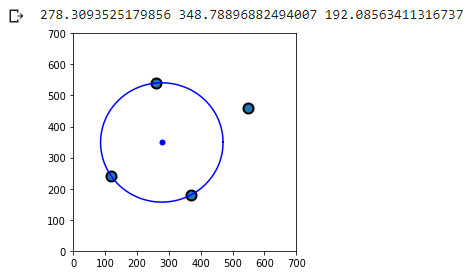
💡 分析运行代码后即可生成外接圆。首先定义三角形列表和外接圆中点、半径的空列表。然后定义了一个名为 circumcircle 的函数该函数接收三个参数即三角形的三个顶点坐标并返回外接圆的中心坐标和半径。调用 circumcircle 函数并将返回值分别赋值给 c_x、c_y 和 radius 变量。然后使用我们刚才介绍的 scatter 函数绘制散点图显示三角形的三个顶点。

对于 circumcircle 函数的实现解析如下

  x = p1[0] + p1[1] * 1j
  y = p2[0] + p2[1] * 1j
  z = p3[0] + p3[1] * 1j

  w = (z - x) / (y - x)
  res = (x - y) * (w - abs(w)**2) / 2j / w.imag - x

  X = -res.real
  Y = -res.imag
  rad = abs(res + x)

  return X, Y, rad

复数运算计算外接圆坐标公式

$\frac{x-y}{y-z}\cdot\frac{x-z}{x-y} = -1$

$res = (x-y)\cdot \left(\frac{x-z}{x-y} - |\frac{x-z}{x-y}|^2\right)/2i/\frac{x-z}{x-y}.imag - x$

解得 $res = -x + 2i \cdot y$ 将 $res$ 展开可得

$\begin{aligned} res = -x + 2i \cdot y\ \Rightarrow X = -res.real, Y = -res.imag \end{aligned}$

其中 $X,Y$ 分别为外接圆的中心点和 $x,y$ 的坐标然后计算外接圆半径

$rad = |res + x|$

最后返回外接圆的中心坐标 $X,Y$ 和半径 $rad$ 。

M = 1000
angle = np.exp(1j * 2 * np.pi / M)
angles = np.cumprod(np.ones(M + 1) * angle)

在绘制外接圆时使用 numpy 中的复数运算函数计算外接圆的坐标。

计算 $M$ 个点的坐标使得这 $M$ 个点组成的曲线恰好是一个外接圆。

angle 表示角度增加的量angles 表示每个角度的值

$angle = e^{i \cdot 2 \pi / M}\, \, \,\, \, \, \, \, \, \, angles = \prod_{i=1}^{M+1} angle$

x = c_x + radius * np.real(angles)  
y = c_y + radius * np.imag(angles)

计算每个点的坐标 $x_i = c_x + rad \cdot \mathrm{real}(angles_i)$ $y_i = c_y + rad \cdot \mathrm{imag}(angles_i)$

其中c_x 和 c_y 分别为外接圆中心点的 $x,y$ 坐标 $rad$ 为外接圆半径 $\mathrm{real}(angles_i)$ 为实部 $\mathrm{imag}(angles_i)$ 为虚部。

plt.plot(x, y, c='b')                      # 绘制外接圆
plt.scatter( [c_x], [c_y], s=25, c= 'b')   # 绘制外接圆中心点

plt.xlim([0, 700])  # 设置x坐标轴范围
plt.ylim([0, 700])  # 设置y坐标轴范围
plt.show()          # 显示图像

最后使用 Matplotlib 中的 plot 函数绘制外接圆再用 scatter 函数绘制外接圆的中心点设置坐标轴的范围show 函数显示图像。

Ⅱ. 德劳内三角剖分Delaunay Triangulation

0x00 引入如何实现德劳内三角剖分

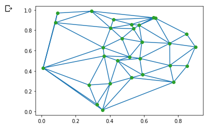
scipy 库提供了现成的 Dealunay 函数供我们使用直接用就行当然你也可以试试手动实现。

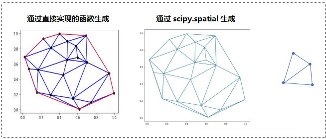
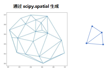
0x01 scipy 库的 Dealunay 函数

介绍SciPy 是一个开源的 Python 算法库和数学工具包。Scipy 是基于 Numpy 的科学计算库用于数学、科学、工程学等领域很多有一些高阶抽象和物理模型需要使用 Scipy。SciPy 包含的模块有最优化、线性代数、积分、插值、特殊函数、快速傅里叶变换、信号处理和图像处理、常微分方程求解和其他科学与工程中常用的计算。

德劳内三角剖分可以通过 scipy 库中的 Delaunay 函数直接生成。

💬 代码演示利用 scipy 库的 Delaunay 函数

import numpy as np
import matplotlib.pyplot as plt
from scipy.spatial import Delaunay

## 随机生成点集
points = np.random.rand(30, 2)

## 计算德劳内使用scipy库中的 Delaunay函数计算
tri = Delaunay(points)

# 画图
plt.triplot(points[:,0], points[:,1], tri.simplices.copy())
plt.plot(points[:,0], points[:,1], 'o')
plt.show()

🚩 运行结果

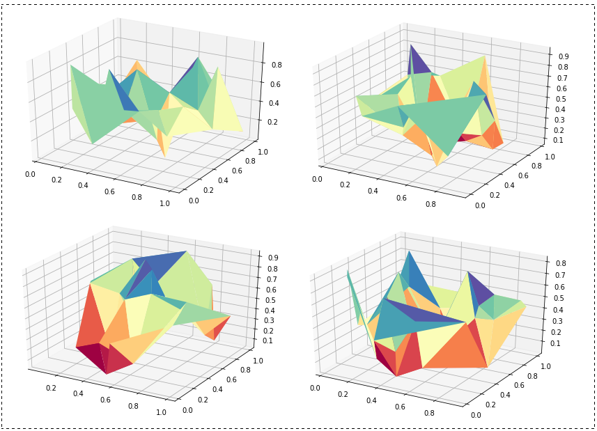
0x02 绘制随机三维立体图形

德劳内三角剖分的应用将立体的表面建模为多边形3D建模

从物体的表面获取许多点后根据这些点进行三角剖分可以最像样地表达立体的形状。

德劳内三角剖分可以通过抓住三个点来表示多边形平面使其接近正三角形因此可以将面积分成一定大小用于三维建模。

由于能够使用尽可能少的三角形来表示物体的表面同时保证三角形的尺寸尽可能均衡。这有助于减少计算量并使建模的结果更加精确。

下面我们就来演示一个简单的 3D 凸立体表面剖分。

🔨 环境准备

!pip install numpy scipy matplotlib scikit-image

💬 代码演示在 3D 坐标系中绘制出剖分后的三角形并绘制随机的三维立体图形。

import numpy as np
from scipy.spatial import Delaunay
import matplotlib.pyplot as plt

points = np.random.rand(30, 3)   # 生成随机的三维坐标点
tri = Delaunay(points)

# 绘制三角剖分后的三维图形
fig = plt.figure()
ax = fig.add_subplot(111, projection='3d')
ax.plot_trisurf (
    points[:,0], 
    points[:,1], 
    points[:,2], 
    triangles=tri.simplices, 
    cmap=plt.cm.Spectral
)
plt.show()

🚩 运行结果运行4次

0x03 计算三角形顶点间距离

德劳内三角剖分的应用设计城市道路网

连接 $n$ 个城市时如果将所有城市和城市直接连接为直线道路。则必须全部建设的道路数为

$nC2=n\, (n-1)\, /\, 2$

实际上可以只连接一些道路使整个城市连接起来。从城市 $A$ 到城市 $B$ 如果没有直接连接的道路可以绕过其他城市。

此时如果要使从城市 $A$ 到城市 $B$ 绕行的总移动距离与 $A-B$ 之间的直线距离相似你就可以使用德劳内三角剖分因为德劳内三角剖分是为了避免出现细长的三角形能够尽量抓住最近的三个点来剖分平面这样可以尽量减少迂回移动距离的增加。

比如将城市坐标点分成多个三角形计算三角形边的距离

import numpy as np
from scipy.spatial import Delaunay

points = np.array (
    [[0,4], [0,1], [1,5], [1,1], [2,0], [2,1]]
)

tri = Delaunay(points)  # 德劳内三角剖分

## 遍历三角形
for i in range(tri.nsimplex):
    indices = tri.simplices[i]   # 获取三角形顶点的下标
    vertices = points[indices]   # 获取顶点坐标
    
    ## 计算顶点之间的距离
    distance = np.linalg.norm(vertices[0] - vertices[1])  \
    + np.linalg.norm(vertices[1] - vertices[2])           \
    + np.linalg.norm(vertices[2] - vertices[0])
    
    ...

得益于德劳内三角剖分的作用使得每个三角形内部的点集在该三角形的内插多项式中都能得到良好的逼近。遍历每个三角形计算三角形的顶点之间的距离。对于每个三角形首可以用 .simplices 获取三角形的顶点下标然后使用这些下标从 points 中获取顶点坐标最后linalg.norm 求范数函数计算两点之间的欧几里得距离。

* 注欧几里得距离公式 $\sqrt{(x_1-x_2)^2+(y_1-y_2)^2}$ 二维空间

Ⅲ. 实战练习Assignment

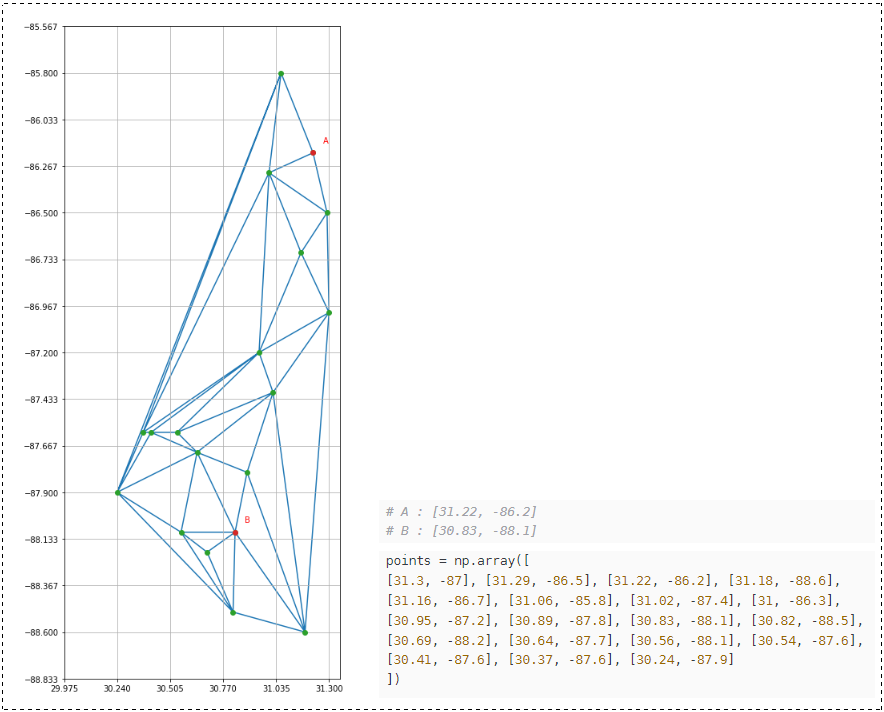
练习A-B 间欧氏距离计算

Google ColaboratoryK80 GPUJupyter Notebookcolab

对于以下给定的点计算输出的每个德劳内三角剖分结果并比较点 $A-B$ 之间的最短距离。

通过识别 $A-B$ 之间的最短路径中包含的点来计算距离手动
计算 $A-B$ 之间的欧氏距离Euclid distance

将 1,2 相比较输出效果如下 *注数据来自于 Dr.Tzeng's Email

🔨 环境准备CV 到 colab 下运行即可

#@title This code cell defines the input data, generates and plots the delaunay triangulation.
from scipy.spatial import Delaunay
import numpy as np
import matplotlib.pyplot as plt
from scipy.interpolate import griddata
from PIL import *
import pandas as pd
import matplotlib.ticker as plticker
import seaborn as sns
!pip install -U scikit-learn

💭 框架提供此代码单元定义输入数据生成并绘制德劳内三角剖分。

grid_size = [5, 13]
fig_size = (30, 15)


# A : [31.22, -86.2]
# B : [30.83, -88.1]


#@title This code cell defines the input data, generates and plots the delaunay triangulation.
from scipy.spatial import Delaunay
import numpy as np
import matplotlib.pyplot as plt
from scipy.interpolate import griddata
from PIL import *
import pandas as pd
import matplotlib.ticker as plticker
import seaborn as sns
!pip install -U scikit-learn

points = np.array([
[31.3, -87], [31.29, -86.5], [31.22, -86.2], [31.18, -88.6],
[31.16, -86.7], [31.06, -85.8], [31.02, -87.4], [31, -86.3], 
[30.95, -87.2], [30.89, -87.8], [30.83, -88.1], [30.82, -88.5], 
[30.69, -88.2], [30.64, -87.7], [30.56, -88.1], [30.54, -87.6], 
[30.41, -87.6], [30.37, -87.6], [30.24, -87.9]
])

values = np.array([5759, 1439, 18827, 20267, 7253, 15893, 2879, 11573, 17387, 
                   4319, 26243, 0, 24641, 21707, 23147, 10133, 8693, 13013, 14453])

norm = np.linalg.norm(values)
norm_values = values / norm

# add the values for each coordinate, and format the data
df = pd.DataFrame(data=points)
df.columns = ['X', 'Y']
df['val'] = values # from the excel sheet
df['norm_val'] = norm_values
x_range, y_range = #TODO

# plot the triangulation
tri = Delaunay(points, incremental=True)
#TODO

# Add the grid
x_ticks = np.arange(df.X.min() - (x_range/(grid_size[0] - 1)), df.X.max() + (x_range/(grid_size[0] - 1)), (x_range/(grid_size[0] - 1)))
y_ticks = np.arange(df.Y.min() - (y_range/(grid_size[1] - 1)), df.Y.max() + (y_range/(grid_size[1] - 1)), (y_range/(grid_size[1] - 1)))
ax.set_xticks(x_ticks)
ax.set_yticks(y_ticks)
ax.set_aspect('equal')
ax.grid()
plt.show()

参考答案

为了不影响练习如需查看答案请自行展开查看



























grid_size = [5, 13]
fig_size = (30, 15)

#@title This code cell defines the input data, generates and plots the delaunay triangulation.
from scipy.spatial import Delaunay
import numpy as np
import matplotlib.pyplot as plt
from scipy.interpolate import griddata
from PIL import *
import pandas as pd
import matplotlib.ticker as plticker
import seaborn as sns
!pip install -U scikit-learn

# using the 19 points from Dr. Tzeng's email.
points = np.array([
[31.3, -87], [31.29, -86.5], [31.22, -86.2], [31.18, -88.6],
[31.16, -86.7], [31.06, -85.8], [31.02, -87.4], [31, -86.3], 
[30.95, -87.2], [30.89, -87.8], [30.83, -88.1], [30.82, -88.5], 
[30.69, -88.2], [30.64, -87.7], [30.56, -88.1], [30.54, -87.6], 
[30.41, -87.6], [30.37, -87.6], [30.24, -87.9]
])

values = np.array([5759, 1439, 18827, 20267, 7253, 15893, 2879, 11573, 17387, 
                   4319, 26243, 0, 24641, 21707, 23147, 10133, 8693, 13013, 14453])

norm = np.linalg.norm(values)
norm_values = values / norm

# 为每个坐标添加值并格式化数据
df = pd.DataFrame(data=points)
df.columns = ['X', 'Y']
df['val'] = values # from the excel sheet
df['norm_val'] = norm_values

x_range = df.X.max() - df.X.min()
y_range = df.Y.max() - df.Y.min()
#TODO

A = [31.22, -86.2]
B = [30.83, -88.1]

axis = np.array([ [ 31.22,-86.2],[ 30.83,-88.1]])# plot the triangulation
tri = Delaunay (points, incremental=True)#TODO
plt.figure(figsize = fig_size)
ax =plt.subplot (111)
ax.triplot (points[ :,0], points [ :,1], tri.simplices.copy())
ax.plot(points[ :,0],points[ :,1], 'o')
ax.plot (axis[:,0], axis[ :,1], 'o')
ax.text(A[ 0]+0.05,A [ 1]+0.05,r"A" ,color = 'R')
ax.text(B[0] + 0.05,B[1] + 0.05, r"B" ,color = 'R')



# Add the grid
x_ticks = np.arange(df.X.min() - (x_range/(grid_size[0] - 1)), df.X.max() + (x_range/(grid_size[0] - 1)), (x_range/(grid_size[0] - 1)))
y_ticks = np.arange(df.Y.min() - (y_range/(grid_size[1] - 1)), df.Y.max() + (y_range/(grid_size[1] - 1)), (y_range/(grid_size[1] - 1)))
ax.set_xticks(x_ticks)
ax.set_yticks(y_ticks)
ax.set_aspect('equal')
ax.grid()
plt.show()

📌 [ 笔者 ]   王亦优
📃 [ 更新 ]   2022.12.21
❌ [ 勘误 ]   /* 暂无 */
📜 [ 声明 ]   由于作者水平有限本文有错误和不准确之处在所难免
              本人也很想知道这些错误恳望读者批评指正

📜 参考资料

Microsoft. MSDN(Microsoft Developer Network)[EB/OL]. []. .

百度百科[EB/OL]. []. https://baike.baidu.com/.

阿里云国内75折回扣微信号：monov8

阿里云国际，腾讯云国际，低至75折。AWS 93折免费开户实名账号代冲值优惠多多微信号：monov8 飞机：@monov6

标签: python

返回列表

上一篇：数据结构—最小生成树_数据结构最小生成树算法

下一篇：【Java 数据结构】队列与OJ题

“【计算几何】德劳内三角剖分算法 | 利用 scatter 绘制散点图 | 实现外接圆生成 | scipy库的 Dealunay 函数 | 实战: A-B间欧氏距离计算_python三维三角剖分” 的相关文章

python基础篇之文件操作1年前 (2023-02-02)

提高Python运行效率的5个技巧!1年前 (2023-02-02)

【阶段三】Python机器学习30篇：机器学习项目实战：智能推荐系统的基本原理与计算相似度的常用方法1年前 (2023-02-02)

python的webdriver应用1年前 (2023-02-02)

Python学习之路-简单语法1年前 (2023-02-02)

Python经典编程习题100例：第36例：求100之内的素数1年前 (2023-02-02)

从0到1【建站:AWS+Ubuntu+Python+Django+uwsgi+nginx+ssl】1年前 (2023-02-02)

【机器学习】贝叶斯算法详解 + 公式推导 + 垃圾邮件过滤实战 + Python代码实现1年前 (2023-02-02)

python 中单下划线和双下划线的区别1年前 (2023-02-02)

Python学习笔记-网络爬虫基础1年前 (2023-02-02)

【计算几何】德劳内三角剖分算法 | 利用 scatter 绘制散点图 | 实现外接圆生成 | scipy库的 Dealunay 函数 | 实战: A-B间欧氏距离计算_python三维三角剖分

Ⅰ. 前置知识

0x00 引入什么是德劳内三角剖分

0x01 学会利用 scatter 函数绘制散点图

0x02 实现外接圆生成函数

Ⅱ. 德劳内三角剖分Delaunay Triangulation

0x00 引入如何实现德劳内三角剖分

0x01 scipy 库的 Dealunay 函数

0x02 绘制随机三维立体图形

0x03 计算三角形顶点间距离

Ⅲ. 实战练习Assignment

练习A-B 间欧氏距离计算

参考答案

“【计算几何】德劳内三角剖分算法 | 利用 scatter 绘制散点图 | 实现外接圆生成 | scipy库的 Dealunay 函数 | 实战: A-B间欧氏距离计算_python三维三角剖分” 的相关文章

阿里云国际版