

机器学习笔记之生成模型综述(二)监督学习与无监督学习
| 阿里云国内75折 回扣 微信号:monov8 |
| 阿里云国际,腾讯云国际,低至75折。AWS 93折 免费开户实名账号 代冲值 优惠多多 微信号:monov8 飞机:@monov6 |
机器学习笔记之生成模型综述——监督学习与无监督学习
引言
上一节介绍了生成模型的判别方式本节将从机器学习需要解决的任务——监督学习、无监督学习的角度对现阶段经典概率模型进行总结。
回顾生成模型介绍
判别方式生成模型 VS \text{VS} VS 判别模型
生成模型( Generative Model \text{Generative Model} Generative Model)的核心判别方式是建模所关注的对象是否在样本分布自身。例如逻辑回归与朴素贝叶斯分类器。虽然这两个算法均处理基于监督学习的分类任务并且均是软分类算法但关注点截然不同
-
逻辑回归( Logistic Regression \text{Logistic Regression} Logistic Regression)的底层逻辑是最大熵原理通过 Sigmoid , Softmax \text{Sigmoid},\text{Softmax} Sigmoid,Softmax函数直接对后验概率 P ( Y ∣ X ) \mathcal P(\mathcal Y \mid \mathcal X) P(Y∣X)进行描述
以二分类为例此时Y \mathcal Y Y服从伯努利分布。
P ( Y ∣ X ) = { Sigmoid ( W T X + b ) Y = 1 1 − Sigmoid ( W T X + b ) Y = 0 \mathcal P(\mathcal Y \mid \mathcal X) = \begin{cases} \text{Sigmoid}(\mathcal W^T\mathcal X + b) \quad \mathcal Y = 1\\ 1 - \text{Sigmoid}(\mathcal W^T\mathcal X + b) \quad \mathcal Y = 0 \end{cases} P(Y∣X)={Sigmoid(WTX+b)Y=11−Sigmoid(WTX+b)Y=0
很明显这里我们仅关注 Sigmoid \text{Sigmoid} Sigmoid函数结果。而 X \mathcal X X得特征信息仅作为与模型参数 W \mathcal W W做内积的一个工具而已并不是我们关注的对象 -
朴素贝叶斯分类器( Naive Bayes Classifier \text{Naive Bayes Classifier} Naive Bayes Classifier)针对后验概率 P ( Y ∣ X ) \mathcal P(\mathcal Y \mid \mathcal X) P(Y∣X)通过贝叶斯定理将其转化为 P ( X ∣ Y ) ⋅ P ( Y ) \mathcal P(\mathcal X \mid \mathcal Y) \cdot \mathcal P(\mathcal Y) P(X∣Y)⋅P(Y)之间的大小关系
关于分母P ( X ) \mathcal P(\mathcal X) P(X)的完整形式是∫ Y P ( X ∣ Y ) ⋅ P ( Y ) d Y \int_{\mathcal Y}\mathcal P(\mathcal X \mid \mathcal Y) \cdot \mathcal P(\mathcal Y) d\mathcal Y ∫YP(X∣Y)⋅P(Y)dY,该项自身与Y \mathcal Y Y无关可视作常数。这里和‘逻辑回归’部分匹配,Y \mathcal Y Y同样服从伯努利分布。
P ( Y ∣ X ) = P ( X , Y ) P ( X ) ∝ P ( X , Y ) = P ( X ∣ Y ) ⋅ P ( Y ) P ( X ∣ Y = 0 ) ⋅ P ( Y = 0 ) ⇔ ? P ( X ∣ Y = 1 ) ⋅ P ( Y = 1 ) \begin{aligned} \mathcal P(\mathcal Y \mid \mathcal X) = \frac{\mathcal P(\mathcal X,\mathcal Y)}{\mathcal P(\mathcal X)} \propto \mathcal P(\mathcal X,\mathcal Y) = \mathcal P(\mathcal X \mid \mathcal Y) \cdot \mathcal P(\mathcal Y) \\ \mathcal P(\mathcal X \mid \mathcal Y = 0) \cdot \mathcal P(\mathcal Y = 0) \overset{\text{?}}{\Leftrightarrow} \mathcal P(\mathcal X \mid \mathcal Y = 1) \cdot \mathcal P(\mathcal Y = 1) \end{aligned} P(Y∣X)=P(X)P(X,Y)∝P(X,Y)=P(X∣Y)⋅P(Y)P(X∣Y=0)⋅P(Y=0)⇔?P(X∣Y=1)⋅P(Y=1)
在这里我们关注的对象是联合概率分布 P ( X , Y ) \mathcal P(\mathcal X,\mathcal Y) P(X,Y)。并且针对 P ( X , Y ) \mathcal P(\mathcal X,\mathcal Y) P(X,Y)建模的过程中设计了条件独立性假设
{ x i ⊥ x j ∣ Y ( i ≠ j ; x i , x j ∈ X ; X ∈ R p ) P ( X ∣ Y ) = P ( x 1 , ⋯ , x p ∣ Y ) = ∏ i = 1 p P ( x i ∣ Y ) \begin{cases} x_i \perp x_j \mid \mathcal Y \quad (i\neq j;x_i,x_j \in \mathcal X;\mathcal X \in \mathbb R^p) \\ \mathcal P(\mathcal X \mid \mathcal Y) = \mathcal P(x_1,\cdots,x_p \mid \mathcal Y) = \prod_{i=1}^p \mathcal P(x_i \mid \mathcal Y) \end{cases} {xi⊥xj∣Y(i=j;xi,xj∈X;X∈Rp)P(X∣Y)=P(x1,⋯,xp∣Y)=∏i=1pP(xi∣Y)
生成模型的建模手段
如果针对监督学习自带标签信息 Y \mathcal Y Y例如朴素贝叶斯分类器通常针对联合概率分布 P ( X , Y ) \mathcal P(\mathcal X,\mathcal Y) P(X,Y)进行建模
如果是无监督学习此时只有样本特征 X \mathcal X X主要分为两种情况
- 例如自回归模型( Autoregressive Model,AR \text{Autoregressive Model,AR} Autoregressive Model,AR)它直接对 P ( X ) \mathcal P(\mathcal X) P(X)自身进行建模
- 隐变量模型( Latent Variable Model,LVM \text{Latent Variable Model,LVM} Latent Variable Model,LVM)通过假设隐变量 Z \mathcal Z Z对联合概率分布 P ( X , Z ) \mathcal P(\mathcal X,\mathcal Z) P(X,Z)进行建模。
监督学习与无监督学习
从机器学习任务的角度观察
- 分类( Classification \text{Classification} Classification)、回归( Regression \text{Regression} Regression) 等明显属于监督学习任务
- 而像降维( Dimensionality Reduction \text{Dimensionality Reduction} Dimensionality Reduction)、聚类( Cluster \text{Cluster} Cluster)、数据生成( Data Generation \text{Data Generation} Data Generation) 等属于无监督学习任务。
无论是监督学习还是无监督学习都可以将其划分为概率模型与非概率模型。
这里的非概率模型自然是指在建模的过程中其关于任务的返回结果没有考虑概率分布。换句话说概率并没有直接参与到相关任务中去。
监督学习模型
基于监督学习的非概率模型
监督学习中的非概率模型大方向指的是判别模型。在分类任务中硬分类模型都是非概率模型。
- 感知机算法(
Perceptron Linear Alpgorithm,PLA
\text{Perceptron Linear Alpgorithm,PLA}
Perceptron Linear Alpgorithm,PLA) 硬分类任务的对应模型均表示特征空间的超平面区别在于样本划分的策略(模型表示后略)
其中Sign \text{Sign} Sign函数表示指示函数。
Y = Sign ( W T X + b ) \mathcal Y = \text{Sign}(\mathcal W^T\mathcal X + b) Y=Sign(WTX+b)
感知机算法的策略是错误驱动
{ L ( W , b ) = ∑ ( x ( i ) , y ( i ) ∈ D ) − y ( i ) ( W T x ( i ) + b ) arg min W , b L ( W , b ) \begin{cases} \mathcal L(\mathcal W,b) = \sum_{(x^{(i)},y^{(i)} \in \mathcal D)} -y^{(i)}\left(\mathcal W^Tx^{(i)} + b \right) \\ \mathop{\arg\min}\limits_{\mathcal W,b} \mathcal L(\mathcal W,b) \end{cases} ⎩ ⎨ ⎧L(W,b)=∑(x(i),y(i)∈D)−y(i)(WTx(i)+b)W,bargminL(W,b) - 硬间隔-支持向量机(
Support Vector Machine,SVM
\text{Support Vector Machine,SVM}
Support Vector Machine,SVM)区别其他的硬分类模型它是一个带约束的优化问题
{ min W , b 1 2 W T W s . t . y ( i ) ( W T x ( i ) + b ) ≥ 1 ( x ( i ) , y ( i ) ) ∈ D \begin{cases} \mathop{\min}\limits_{\mathcal W,b} \frac{1}{2}\mathcal W^T\mathcal W \\ s.t. y^{(i)} \left(\mathcal W^Tx^{(i)} + b\right) \geq 1 \quad (x^{(i)},y^{(i)}) \in \mathcal D \end{cases} ⎩ ⎨ ⎧W,bmin21WTWs.t.y(i)(WTx(i)+b)≥1(x(i),y(i))∈D - 线性判别分析(
Linear Discriminant Analysis,LDA
\text{Linear Discriminant Analysis,LDA}
Linear Discriminant Analysis,LDA)以二分类为例通过描述被超平面划分样本点的类内、类间关系来确定模型参数信息。其策略表示如下
J ( W ) = ( Z 1 ˉ − Z 2 ) 2 ˉ S 1 + S 2 = W T ( X C 1 ˉ − X C 2 ˉ ) ( X C 1 ˉ − X C 2 ˉ ) T W W T ( S C 1 + S C 2 ) W { S C 1 = 1 N 1 ∑ i = 1 N 1 ( x ( i ) − X C 1 ˉ ) ( x ( i ) − X C 1 ˉ ) T X C 1 ˉ = 1 N 1 ∑ i = 1 N 1 x ( i ) \begin{aligned} \mathcal J(\mathcal W) & = \frac{(\bar{\mathcal Z_1} - \bar{\mathcal Z_2)^2}}{\mathcal S_1 + \mathcal S_2} \\ & = \frac{\mathcal W^T(\bar{\mathcal X_{\mathcal C_1}} - \bar{\mathcal X_{\mathcal C_2}})(\bar{\mathcal X_{\mathcal C_1}} - \bar{\mathcal X_{\mathcal C_2}})^T \mathcal W}{\mathcal W^T(\mathcal S_{\mathcal C_1} + \mathcal S_{\mathcal C_2}) \mathcal W} \\ & \begin{cases} \mathcal S_{\mathcal C_1} = \frac{1}{N_1} \sum_{i=1}^{N_1} (x^{(i)} - \bar{\mathcal X_{\mathcal C_1}})(x^{(i)} - \bar{\mathcal X_{\mathcal C_1}})^T \\ \bar {\mathcal X_{\mathcal C_1}} = \frac{1}{N_1} \sum_{i=1}^{N_1} x^{(i)} \end{cases} \end{aligned} J(W)=S1+S2(Z1ˉ−Z2)2ˉ=WT(SC1+SC2)WWT(XC1ˉ−XC2ˉ)(XC1ˉ−XC2ˉ)TW{SC1=N11∑i=1N1(x(i)−XC1ˉ)(x(i)−XC1ˉ)TXC1ˉ=N11∑i=1N1x(i) - 多层感知机/前馈神经网络(
Feed-Forword Neural Network
\text{Feed-Forword Neural Network}
Feed-Forword Neural Network)其核心是通用逼近定理。
- 关于神经网络处理硬分类问题例如亦或问题可以将其视作非概率判别模型
基于亦或问题的前馈神经网络结构表示如下。
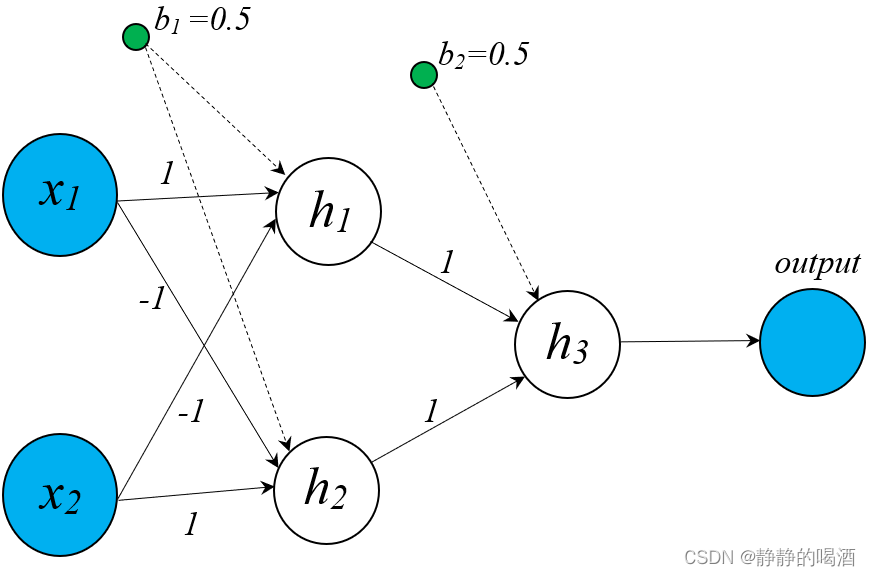
- 如果是软分类问题如在网络输出层加上 Sigmoid,Softmax \text{Sigmoid,Softmax} Sigmoid,Softmax函数作为输出它此时被视作概率判别模型。
- 如果是回归任务并不称其为判别模型能够确定的是它是一个非概率模型。
- 关于神经网络处理硬分类问题例如亦或问题可以将其视作非概率判别模型
- 除了基于直线/超平面形状的硬分类算法还如其他算法如决策树( Decision Tree \text{Decision Tree} Decision Tree)等其他树模型也属于监督学习中的非概率模型。
基于监督学习的概率模型
监督学习中的概率模型可以继续向下划分可划分为概率判别模型( Discriminative Model \text{Discriminative Model} Discriminative Model)和概率生成模型( Generative Model \text{Generative Model} Generative Model)两种
-
其中概率判别模型的核心思想是直接对条件概率 P ( Y ∣ X ) \mathcal P(\mathcal Y \mid \mathcal X) P(Y∣X)进行建模 。经典的概率判别模型有
- 逻辑回归(
Logistic Regression,LR
\text{Logistic Regression,LR}
Logistic Regression,LR)它的模型结构与其他分类任务的非概率模型相同均是特征空间的直线/超平面
这里的Sign \text{Sign} Sign函数指的是Sigmoid \text{Sigmoid} Sigmoid函数自身。
Y = Sigmoid ( W T X + b ) \mathcal Y = \text{Sigmoid}(\mathcal W^T\mathcal X + b) Y=Sigmoid(WTX+b)
假设标签信息 Y \mathcal Y Y服从伯努利分布逻辑回归使用 Sigmoid \text{Sigmoid} Sigmoid函数直接对 P ( Y ∣ X ) \mathcal P(\mathcal Y \mid \mathcal X) P(Y∣X)进行表达
其中W , b \mathcal W,b W,b分别表示权重参数与偏置信息。
P ( Y ∣ X ) = { Sigmoid ( W T X + b ) Y = 1 1 − Sigmoid ( W T X + b ) Y = 0 \mathcal P(\mathcal Y \mid \mathcal X) = \begin{cases} \text{Sigmoid}(\mathcal W^T\mathcal X + b) \quad \mathcal Y = 1 \\ 1 - \text{Sigmoid}(\mathcal W^T\mathcal X + b) \quad \mathcal Y = 0 \end{cases} P(Y∣X)={Sigmoid(WTX+b)Y=11−Sigmoid(WTX+b)Y=0 - 最大熵马尔可夫模型(
Maximum Entropy Markov Model,MEMM
\text{Maximum Entropy Markov Model,MEMM}
Maximum Entropy Markov Model,MEMM)该模型的概率图结构表示如下
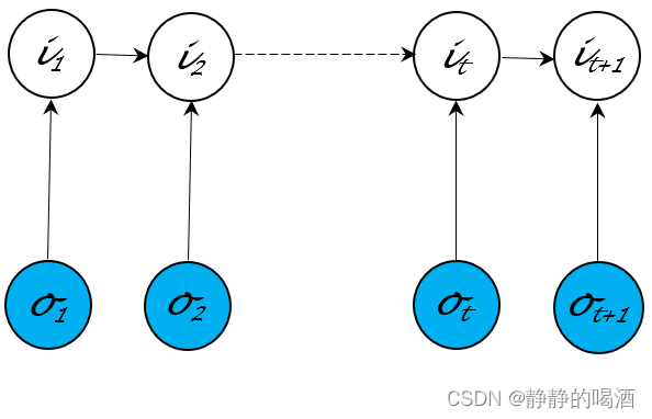
这种概率图结构打破了观测独立性假设的约束。并且它直接对隐变量 I \mathcal I I的后验概率进行建模
P ( I ∣ O ; λ ) = P ( i 1 , ⋯ , i T ∣ o 1 , ⋯ , o T ; λ ) = P ( i 1 ∣ o 1 ; λ ) ⋅ ∏ t = 2 T P ( i t ∣ i t − 1 , o t ; λ ) \begin{aligned} \mathcal P(\mathcal I \mid \mathcal O;\lambda) & = \mathcal P(i_1,\cdots,i_{T} \mid o_1,\cdots,o_{T};\lambda) \\ & = \mathcal P(i_1 \mid o_1;\lambda) \cdot \prod_{t=2}^{T} \mathcal P(i_t \mid i_{t-1},o_t;\lambda) \end{aligned} P(I∣O;λ)=P(i1,⋯,iT∣o1,⋯,oT;λ)=P(i1∣o1;λ)⋅t=2∏TP(it∣it−1,ot;λ) - 条件随机场(
Condition Random Field,CRF
\text{Condition Random Field,CRF}
Condition Random Field,CRF) 该模型的概率图结构表示如下
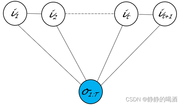
在给定观测变量 O \mathcal O O的条件下直接对 P ( I ∣ O ) \mathcal P(\mathcal I \mid \mathcal O) P(I∣O)进行建模
关于这种链式的无向图结构它的极大团内仅包含相邻的两个随机变量结点与观测变量结点这里将极大团数量K \mathcal K K替换为序列长度T T T;并且− E k ( i C k ) -\mathbb E_{k}(i_{\mathcal C_k}) −Ek(iCk)表示能量函数恒正;Z \mathcal Z Z表示配分函数。
P ( I ∣ O ) = 1 Z exp ∑ k = 1 K − E k ( i C k ) = 1 Z exp ∑ t = 1 T f t ( i t , i t + 1 , O ) \begin{aligned} \mathcal P(\mathcal I \mid \mathcal O) & = \frac{1}{\mathcal Z} \exp \sum_{k=1}^{\mathcal K} - \mathbb E_{k}(i_{\mathcal C_k}) \\ & = \frac{1}{\mathcal Z} \exp \sum_{t=1}^{T}f_t(i_t,i_{t+1},\mathcal O) \end{aligned} P(I∣O)=Z1expk=1∑K−Ek(iCk)=Z1expt=1∑Tft(it,it+1,O)
从上述介绍的几种模型也能观察到并不能将所有的隐变量模型武断地看作生成模型对于判别模型与生成模型的界限存在新的认识。
- 逻辑回归(
Logistic Regression,LR
\text{Logistic Regression,LR}
Logistic Regression,LR)它的模型结构与其他分类任务的非概率模型相同均是特征空间的直线/超平面
无监督学习
基于无监督学习的概率模型
由于无监督学习中没有标签信息仅包含样本特征因此无法通过标签信息进行判别。因而基于无监督的概率模型只有概率生成模型。
这里所说的概率分布只会是样本
X
\mathcal X
X的概率分布。
基于无监督学习的非概率模型
关于无监督学习的非概率模型主要针对于特定任务。如
- 降维-主成分分析(
Principal Component Analysis,PCA
\text{Principal Component Analysis,PCA}
Principal Component Analysis,PCA)在执行去中心化操作后找到主成分
u
⃗
\vec u
u使
u
⃗
\vec u
u满足如下条件
{ u ^ = arg max u ⃗ J { J = u ⃗ T ⋅ [ 1 N ∑ i = 1 N ( x ( i ) − X ˉ ) ( x ( i ) − X ˉ ) T ] ⋅ u ⃗ X ˉ = 1 N ∑ i = 1 N x ( i ) s . t . u ⃗ T ⋅ u ⃗ = 1 \begin{cases} \hat u = \mathop{\arg\max}\limits_{\vec u} \mathcal J \quad \begin{cases} \mathcal J = \vec u^T \cdot \left[\frac{1}{N} \sum_{i=1}^N(x^{(i)} - \bar {\mathcal X})(x^{(i)} - \bar {\mathcal X})^T \right] \cdot \vec u \\ \bar {\mathcal X} = \frac{1}{N} \sum_{i=1}^N x^{(i)} \end{cases}\\ s.t. \quad \vec u^T \cdot \vec u = 1 \\ \end{cases} ⎩ ⎨ ⎧u^=uargmaxJ{J=uT⋅[N1∑i=1N(x(i)−Xˉ)(x(i)−Xˉ)T]⋅uXˉ=N1∑i=1Nx(i)s.t.uT⋅u=1 - 其他的非概率模型如用于聚类任务的 K-means \text{K-means} K-means自编码器等等。
生成模型介绍
关于生成模型将其从监督任务、非监督任务进行划分意义不大。因而统一进行描述。首先需要排除一些错误认知
- 概率图模型特别是隐变量模型并不全是生成模型。
如上面介绍的最大熵马尔可夫模型、条件随机场它们是判别模型。只能说概率图模型中的大部分模型是生成模型。 - 相反生成模型也并不全是概率图模型例如神经网络。
- 在处理回归任务中前馈神经网络结构可以视作非概率模型。如线性回归( Linear Regression \text{Linear Regression} Linear Regression)
- 在处理硬分类任务中如前馈神经网络处理亦或问题此时的前馈神经网络结构可以视作非概率的判别模型
- 在处理软分类任务如逻辑回归此时的前馈神经网络结构可以视作概率判别模型
- 在无监督学习任务中针对非概率模型有自编码器( Auto-Encoder \text{Auto-Encoder} Auto-Encoder)
- 基于神经网络的分布式表示思想通过神经网络实现特征提取此时的神经网络可以被划分至概率生成模型。
也就是说生成模型横跨了概率图模型以及深度学习特别是将神经网络与概率图模型混合的产物——深度生成模型( Deep Generative Model \text{Deep Generative Model} Deep Generative Model)
-
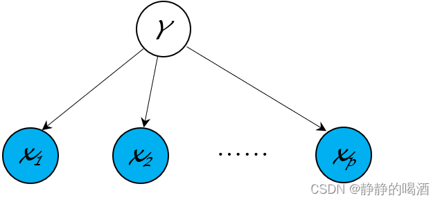
在介绍的生成模型中假设最简单的生成模型——朴素贝叶斯分类器( Naive Bayes Classifier \text{Naive Bayes Classifier} Naive Bayes Classifier)它的核心是朴素贝叶斯假设
x i ⊥ x j ∣ Y = l { i , j ∈ { 1 , 2 , ⋯ , p } / X ∈ R p i ≠ j l ∈ { 1 , 2 , ⋯ , k } x_i \perp x_j \mid \mathcal Y = l \quad \begin{cases} i,j \in \{1,2,\cdots,p\} / \mathcal X \in \mathbb R^p \\ i \neq j \\ l \in \{1,2,\cdots,k\} \end{cases} xi⊥xj∣Y=l⎩ ⎨ ⎧i,j∈{1,2,⋯,p}/X∈Rpi=jl∈{1,2,⋯,k}
主要应用在监督学习的分类任务对应的概率图结构表示如下
很明显它并不是混合模型。x 1 , ⋯ , x p x_1,\cdots,x_p x1,⋯,xp是随机变量表示样本自身的各维度特征;Y \mathcal Y Y表示样本对应的标签信息。
-
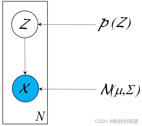
混合模型系列仅通过样本自身特征信息无法准确描述概率分布需要引入隐变量 Z \mathcal Z Z进行建模。如高斯混合模型( Gaussian Mixture Model,GMM \text{Gaussian Mixture Model,GMM} Gaussian Mixture Model,GMM)其中 Z \mathcal Z Z被假设为一维、离散型随机变量并且 X ∣ Z \mathcal X \mid \mathcal Z X∣Z服从高斯分布
根据实际情况也可以将其设置为其他分布构建不同的混合模型。
X ∣ Z ∼ N ( μ k , Σ k ) \mathcal X \mid \mathcal Z \sim \mathcal N(\mu_{k},\Sigma_{k}) X∣Z∼N(μk,Σk)
对应的建模过程表示为
关于包含隐变量生成模型的建模过程主要是对联合概率分布P ( X , Z ) \mathcal P(\mathcal X,\mathcal Z) P(X,Z)进行建模。
P ( X ) = ∑ Z P ( X , Z ) = ∑ Z P ( X ∣ Z ) ⋅ P ( Z ) = ∑ k = 1 K p k ⋅ N ( μ k , Σ k ) ( ∑ k = 1 K p k = 1 ) \begin{aligned} \mathcal P(\mathcal X) & = \sum_{\mathcal Z} \mathcal P(\mathcal X,\mathcal Z) \\ & = \sum_{\mathcal Z} \mathcal P(\mathcal X \mid \mathcal Z) \cdot \mathcal P(\mathcal Z) \\ & = \sum_{k=1}^{\mathcal K} p_{k} \cdot \mathcal N(\mu_{k},\Sigma_{k}) \quad (\sum_{k=1}^{\mathcal K} p_k = 1) \end{aligned} P(X)=Z∑P(X,Z)=Z∑P(X∣Z)⋅P(Z)=k=1∑Kpk⋅N(μk,Σk)(k=1∑Kpk=1)
主要应用在无监督学习的聚类任务。其概率图结构表示如下
-
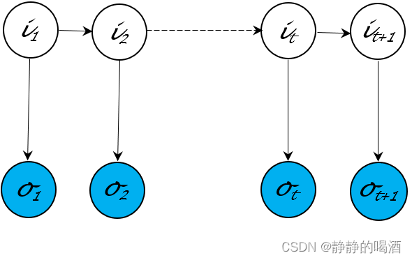
动态模型( Dynamic Model \text{Dynamic Model} Dynamic Model)系列从时间、序列角度随机变量从有限到无限。代表模型有隐马尔可夫模型( Hidden Markov Model,HMM \text{Hidden Markov Model,HMM} Hidden Markov Model,HMM)卡尔曼滤波( Kalman Filter \text{Kalman Filter} Kalman Filter)粒子滤波( Praticle Filter \text{Praticle Filter} Praticle Filter)。它们均服从齐次马尔可夫假设与观测独立性假设
{ P ( i t + 1 ∣ i t , ⋯ ) = P ( i t + 1 ∣ i t ) P ( o t ∣ i t , ⋯ ) = P ( o t ∣ i t ) \begin{cases} \mathcal P(i_{t+1} \mid i_t,\cdots) = \mathcal P(i_{t+1} \mid i_t) \\ \mathcal P(o_t \mid i_t,\cdots) = \mathcal P(o_t \mid i_t) \end{cases} {P(it+1∣it,⋯)=P(it+1∣it)P(ot∣it,⋯)=P(ot∣it)
对应的概率图结构表示如下
-
从空间角度的随机变量从有限到无限代表模型有高斯过程( Gaussian Process \text{Gaussian Process} Gaussian Process)准确的说高斯过程是联合正态分布的无限维的广义延伸主要应用在高维的非线性回归任务中
由于连续域中的片段是无法划分完的因此仅示例N N N个重要片段。
后续补充:狄利克雷过程~
{ ξ t } t ∈ T = { ξ t 1 , ξ t 2 , ⋯ , ξ t N } ⏟ N 个重要片段 { ξ t 1 ∼ N ( μ t 1 , Σ t 1 ) ξ t 2 ∼ N ( μ t 2 , Σ t 2 ) ⋯ ξ t N ∼ N ( μ t N , Σ t N ) \left\{\xi_t\right\}_{t \in \mathcal T} = \underbrace{\{\xi_{t_1},\xi_{t_2},\cdots,\xi_{t_{N}}\}}_{N个重要片段} \quad \begin{cases} \xi_{t_1} \sim \mathcal N(\mu_{t_1},\Sigma_{t_1}) \\ \xi_{t_2} \sim \mathcal N(\mu_{t_2},\Sigma_{t_2}) \\ \cdots \\ \xi_{t_N} \sim \mathcal N(\mu_{t_N},\Sigma_{t_N}) \\ \end{cases} {ξt}t∈T=N个重要片段 {ξt1,ξt2,⋯,ξtN}⎩ ⎨ ⎧ξt1∼N(μt1,Σt1)ξt2∼N(μt2,Σt2)⋯ξtN∼N(μtN,ΣtN)- 对比于高斯分布仅需要知道该分布的参数(均值、方差)就可以确定一个高斯分布
- 高斯过程中连续域中的任意一个片段均服从一个高斯分布它的参数可能是无限个。如高斯过程这种参数空间从有限到无限的模型被称作 非参数贝叶斯模型( Non-Parameter Bayessian Model \text{Non-Parameter Bayessian Model} Non-Parameter Bayessian Model)。
-
以隐狄利克雷分配( Latent Dirichlet Allocation,LDA \text{Latent Dirichlet Allocation,LDA} Latent Dirichlet Allocation,LDA)为代表的 Mixed Memership Model \text{Mixed Memership Model} Mixed Memership Model。
-
以因子分析( Factorial Analysis,FA \text{Factorial Analysis,FA} Factorial Analysis,FA)为代表的因子模型( Factorial Model \text{Factorial Model} Factorial Model)其他模型有概率性主成分分析( Probabilistic Principal Component Analysis,P-PCA \text{Probabilistic Principal Component Analysis,P-PCA} Probabilistic Principal Component Analysis,P-PCA)等。
后续模型就是概率图模型与深度学习相结合的概率生成模型——深度生成模型。
- 以玻尔兹曼机(
Boltzmann Machine,BM
\text{Boltzmann Machine,BM}
Boltzmann Machine,BM)为代表的能量模型(
Energy-based Model
\text{Energy-based Model}
Energy-based Model)。玻尔兹曼机的概率图结构表示如下
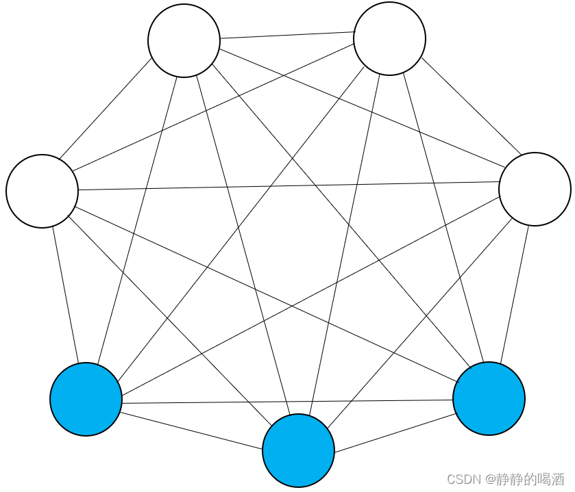
对应的模型表示为(对联合概率分布 P ( v , h ) \mathcal P(v,h) P(v,h)进行建模。下同)
其中v T R ⋅ v ; h T S ⋅ h ; v T W ⋅ h v^T \mathcal R \cdot v;h^T\mathcal S \cdot h;v^T\mathcal W \cdot h vTR⋅v;hTS⋅h;vTW⋅h分别表示包含边相关联结点之间的能量表达;b T v ; c T h b^Tv;c^Th bTv;cTh分别表示各结点内部的能量表达(b , c b,c b,c可看作偏置信息)
P ( v , h ) = 1 Z exp { − E [ v , h ] } = 1 Z exp { [ v T R ⋅ v + b T v + v T W ⋅ h + h T S ⋅ h + c T h ] } \begin{aligned} \mathcal P(v,h) & = \frac{1}{\mathcal Z} \exp \{- \mathbb E [v,h]\} \\ & = \frac{1}{\mathcal Z} \exp \{\left[v^T \mathcal R \cdot v + b^T v + v^T \mathcal W \cdot h + h^T\mathcal S \cdot h + c^Th\right]\} \end{aligned} P(v,h)=Z1exp{−E[v,h]}=Z1exp{[vTR⋅v+bTv+vTW⋅h+hTS⋅h+cTh]}
其中包括受限玻尔兹曼机( Restricted Boltzmann Machine,RBM \text{Restricted Boltzmann Machine,RBM} Restricted Boltzmann Machine,RBM)对应概率图结构表示如下
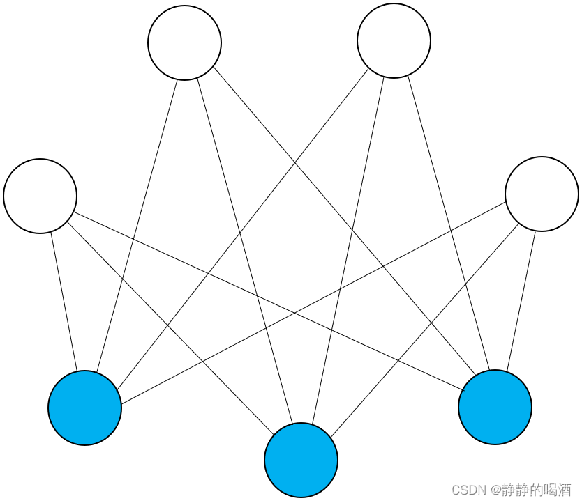
对应模型表示为
和玻尔兹曼机相比受限玻尔兹曼机隐变量、观测变量内部各随机变量相互独立。
P ( v , h ) = 1 Z exp { − E ( v , h ) } = 1 Z exp ( v T W ⋅ h + b T v + c T h ) \begin{aligned} \mathcal P(v,h) & = \frac{1}{\mathcal Z} \exp \{-\mathbb E(v,h)\} \\ & = \frac{1}{\mathcal Z} \exp (v^T\mathcal W \cdot h + b^Tv + c^Th) \end{aligned} P(v,h)=Z1exp{−E(v,h)}=Z1exp(vTW⋅h+bTv+cTh)
Sigmoid \text{Sigmoid} Sigmoid信念网络( Sigmoid Belief Network \text{Sigmoid Belief Network} Sigmoid Belief Network)它的概率图结构表示如下
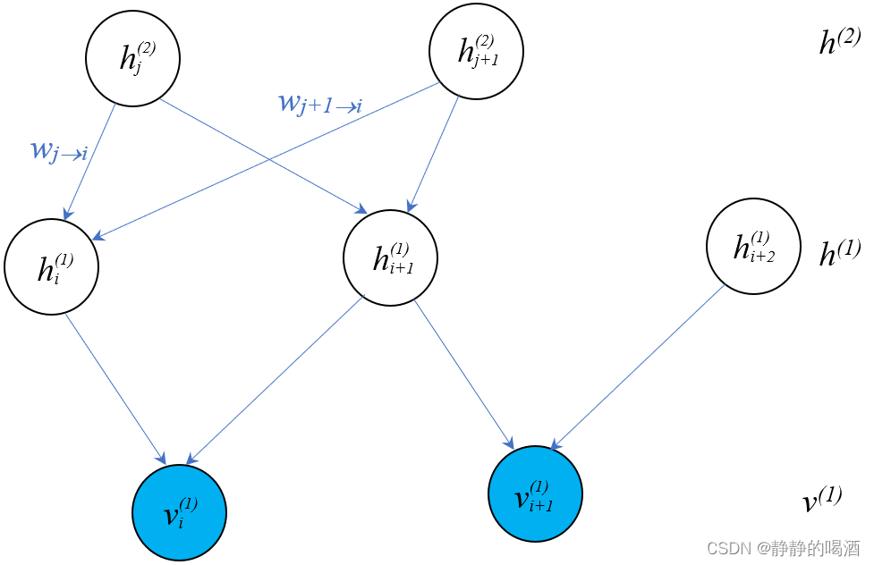
对应模型表示为
由于Sigmoid \text{Sigmoid} Sigmoid信念网络是有向图模型因而可以通过结点之间的因果关系对模型进行表示。
P ( v , h ) = P ( v i ( 1 ) , v i + 1 ( 1 ) , h i ( 1 ) , h i + 1 ( 1 ) , h i + 2 ( 1 ) , h j ( 2 ) , h j + 1 ( 2 ) ) = P ( h j ( 2 ) ) ⋅ P ( h j + 1 ( 2 ) ) ⋅ P ( h i ( 1 ) ∣ h j ( 2 ) , h j + 1 ( 2 ) ) ⋅ P ( h i + 1 ( 1 ) ∣ h j ( 2 ) , h j + 1 ( 2 ) ) ⋅ P ( v i ( 1 ) ∣ h i ( 1 ) , h i + 1 ( 1 ) ) ⋅ P ( h i + 2 ( 1 ) ) ⋅ P ( v i + 1 ( 1 ) ∣ h i + 1 ( 1 ) , h i + 2 ( 1 ) ) \begin{aligned} \mathcal P(v,h) & = \mathcal P (v_i^{(1)},v_{i+1}^{(1)},h_{i}^{(1)},h_{i+1}^{(1)},h_{i+2}^{(1)},h_{j}^{(2)},h_{j+1}^{(2)}) \\ & = \mathcal P(h_j^{(2)}) \cdot \mathcal P(h_{j+1}^{(2)}) \cdot \mathcal P(h_{i}^{(1)} \mid h_{j}^{(2)},h_{j+1}^{(2)}) \cdot \mathcal P(h_{i+1}^{(1)} \mid h_{j}^{(2)},h_{j+1}^{(2)}) \cdot \mathcal P(v_i^{(1)} \mid h_{i}^{(1)},h_{i+1}^{(1)}) \cdot \mathcal P(h_{i+2}^{(1)}) \cdot \mathcal P(v_{i+1}^{(1)} \mid h_{i+1}^{(1)},h_{i+2}^{(1)}) \end{aligned} P(v,h)=P(vi(1),vi+1(1),hi(1),hi+1(1),hi+2(1),hj(2),hj+1(2))=P(hj(2))⋅P(hj+1(2))⋅P(hi(1)∣hj(2),hj+1(2))⋅P(hi+1(1)∣hj(2),hj+1(2))⋅P(vi(1)∣hi(1),hi+1(1))⋅P(hi+2(1))⋅P(vi+1(1)∣hi+1(1),hi+2(1))
深度信念网络( Deep Belief Network,DBN \text{Deep Belief Network,DBN} Deep Belief Network,DBN)它的概率图结构表示如下
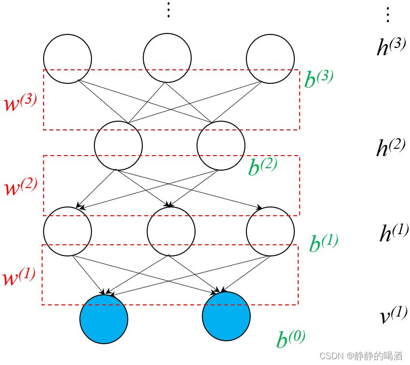
对应模型表示为
P ( v ( 1 ) , h ( 1 ) , h ( 2 ) , h ( 3 ) ) = ∏ i = 1 D P ( v i ( 1 ) ∣ h ( 1 ) ) ⋅ ∏ j = 1 P ( 1 ) P ( h j ( 1 ) ∣ h ( 2 ) ) ⋅ P ( h ( 2 ) , h ( 3 ) ) { P ( v i ( 1 ) ∣ h ( 1 ) ) = Sigmoid { [ W h ( 1 ) → v i ( 1 ) ] T h ( 1 ) + b i ( 0 ) } [ W h ( 1 ) → v i ( 1 ) ] P ( 1 ) × 1 ∈ W ( 1 ) P ( h j ( 1 ) ∣ h ( 2 ) ) = Sigmoid { [ W h ( 2 ) → h j ( 1 ) ] T h ( 2 ) + b j ( 1 ) } [ W h ( 2 ) → h j ( 1 ) ] P ( 2 ) × 1 ∈ W ( 2 ) P ( h ( 2 ) , h ( 3 ) ) = 1 Z exp { [ h ( 3 ) ] T W ( 3 ) ⋅ h ( 2 ) + [ h ( 2 ) ] T ⋅ b ( 2 ) + [ h ( 3 ) ] T b ( 3 ) } \begin{aligned} & \mathcal P(v^{(1)},h^{(1)},h^{(2)},h^{(3)}) = \prod_{i=1}^{\mathcal D} \mathcal P(v_i^{(1)} \mid h^{(1)}) \cdot \prod_{j=1}^{\mathcal P^{(1)}} \mathcal P(h_j^{(1)} \mid h^{(2)}) \cdot \mathcal P(h^{(2)},h^{(3)}) \\ & \begin{cases} \mathcal P(v_i^{(1)} \mid h^{(1)}) = \text{Sigmoid} \left\{\left[\mathcal W_{h^{(1)} \to v_i^{(1)}}\right]^T h^{(1)} + b_i^{(0)}\right\} \quad \left[\mathcal W_{h^{(1)} \to v_i^{(1)}}\right]_{\mathcal P^{(1)} \times 1} \in \mathcal W^{(1)} \\ \mathcal P(h_j^{(1)} \mid h^{(2)}) = \text{Sigmoid} \left\{\left[\mathcal W_{h^{(2)} \to h_j^{(1)}}\right]^T h^{(2)} + b_j^{(1)}\right\} \quad \left[\mathcal W_{h^{(2)} \to h_j^{(1)}}\right]_{\mathcal P^{(2)} \times 1} \in \mathcal W^{(2)} \\ \mathcal P(h^{(2)},h^{(3)}) = \frac{1}{\mathcal Z} \exp \left\{ \left[h^{(3)}\right]^T \mathcal W^{(3)} \cdot h^{(2)} + \left[h^{(2)}\right]^T\cdot b^{(2)} + \left[h^{(3)}\right]^Tb^{(3)}\right\} \\ \end{cases} \end{aligned} P(v(1),h(1),h(2),h(3))=i=1∏DP(vi(1)∣h(1))⋅j=1∏P(1)P(hj(1)∣h(2))⋅P(h(2),h(3))⎩ ⎨ ⎧P(vi(1)∣h(1))=Sigmoid{[Wh(1)→vi(1)]Th(1)+bi(0)}[Wh(1)→vi(1)]P(1)×1∈W(1)P(hj(1)∣h(2))=Sigmoid{[Wh(2)→hj(1)]Th(2)+bj(1)}[Wh(2)→hj(1)]P(2)×1∈W(2)P(h(2),h(3))=Z1exp{[h(3)]TW(3)⋅h(2)+[h(2)]T⋅b(2)+[h(3)]Tb(3)}
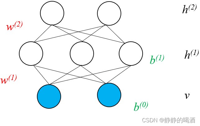
深度玻尔兹曼机( Deep Boltzmann Machine,DBM \text{Deep Boltzmann Machine,DBM} Deep Boltzmann Machine,DBM)它的概率图结构表示如下
- 将神经网络与概率相结合的生成模型。
如变分自编码器( Variational Auto-Encoder,VAE \text{Variational Auto-Encoder,VAE} Variational Auto-Encoder,VAE)它的概率图结构依然是混合模型(引入隐变量模型)的概率图结构。
生成对抗网络( Generative Adversarial Networks,GAN \text{Generative Adversarial Networks,GAN} Generative Adversarial Networks,GAN)其计算图结构表示如下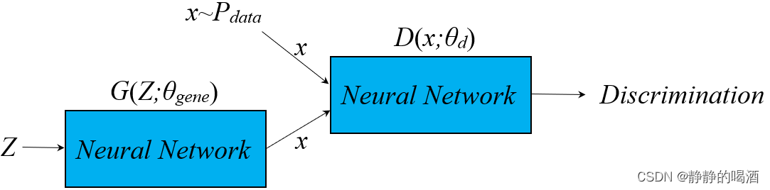
以及流模型( Flow-based Model \text{Flow-based Model} Flow-based Model)和自回归模型( Autoregressive Model \text{Autoregressive Model} Autoregressive Model)。
相关参考
生成模型2-监督VS非监督