

垃圾邮件(短信)分类算法实现 机器学习 深度学习 计算机竞赛-CSDN博客
| 阿里云国内75折 回扣 微信号:monov8 |
| 阿里云国际,腾讯云国际,低至75折。AWS 93折 免费开户实名账号 代冲值 优惠多多 微信号:monov8 飞机:@monov6 |
文章目录
0 前言
优质竞赛项目系列今天要分享的是
垃圾邮件(短信)分类算法实现 机器学习 深度学习
该项目较为新颖适合作为竞赛课题方向学长非常推荐
学长这里给一个题目综合评分(每项满分5分)
- 难度系数3分
- 工作量3分
- 创新点4分
更多资料, 项目分享
https://gitee.com/dancheng-senior/postgraduate
2 垃圾短信/邮件 分类算法 原理
垃圾邮件内容往往是广告或者虚假信息甚至是电脑病毒、情色、反动等不良信息大量垃圾邮件的存在不仅会给人们带来困扰还会造成网络资源的浪费
网络舆情是社会舆情的一种表现形式网络舆情具有形成迅速、影响力大和组织发动优势强等特点网络舆情的好坏极大地影响着社会的稳定通过提高舆情分析能力有效获取发布舆论的性质避免负面舆论的不良影响是互联网面临的严肃课题。
将邮件分为垃圾邮件(有害信息)和正常邮件网络舆论分为负面舆论(有害信息)和正面舆论那么无论是垃圾邮件过滤还是网络舆情分析都可看作是短文本的二分类问题。
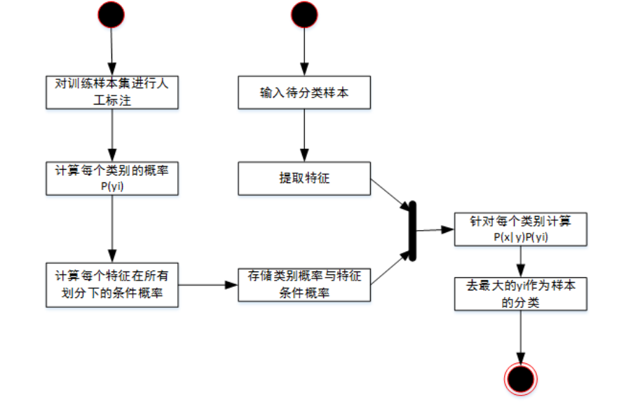
2.1 常用的分类器 - 贝叶斯分类器
贝叶斯算法解决概率论中的一个典型问题一号箱子放有红色球和白色球各 20 个二号箱子放油白色球 10 个红色球 30
个。现在随机挑选一个箱子取出来一个球的颜色是红色的请问这个球来自一号箱子的概率是多少
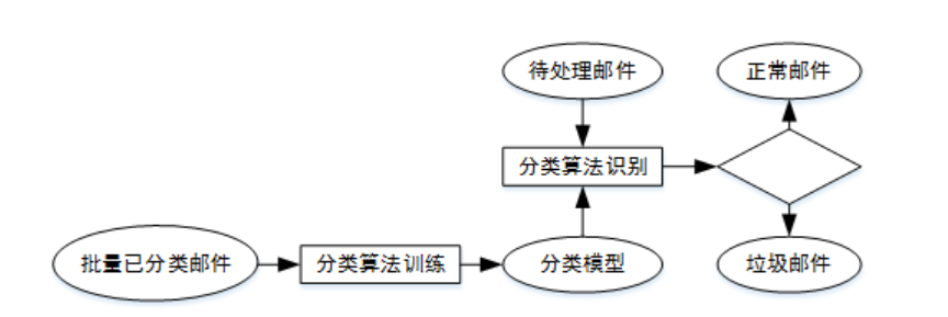
利用贝叶斯算法识别垃圾邮件基于同样道理根据已经分类的基本信息获得一组特征值的概率如“茶叶”这个词出现在垃圾邮件中的概率和非垃圾邮件中的概率就得到分类模型然后对待处理信息提取特征值结合分类模型判断其分类。
贝叶斯公式
P(B|A)=P(A|B)*P(B)/P(A)
P(B|A)=当条件 A 发生时B 的概率是多少。代入当球是红色时来自一号箱的概率是多少
P(A|B)=当选择一号箱时,取出红色球的概率。
P(B)=一号箱的概率。
P(A)=取出红球的概率。
代入垃圾邮件识别
P(B|A)=当包含"茶叶"这个单词时是垃圾邮件的概率是多少
P(A|B)=当邮件是垃圾邮件时包含“茶叶”这个单词的概率是多少
P(B)=垃圾邮件总概率。
P(A)=“茶叶”在所有特征值中出现的概率。
3 数据集介绍
使用中文邮件数据集丹成学长自己采集通过爬虫以及人工筛选。
数据集“data” 文件夹中包含“full” 文件夹和 “delay” 文件夹。
“data” 文件夹里面包含多个二级文件夹二级文件夹里面才是垃圾邮件文本一个文本代表一份邮件。“full” 文件夹里有一个 index
文件该文件记录的是各邮件文本的标签。
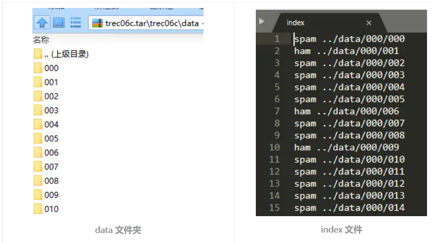
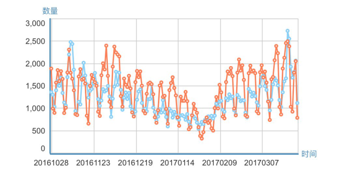
数据集可视化
4 数据预处理
这一步将分别提取邮件样本和样本标签到一个单独文件中顺便去掉邮件的非中文字符将邮件分好词。
邮件大致内容如下图
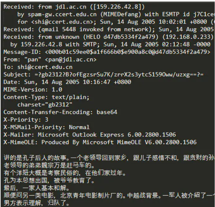
每一个邮件样本除了邮件文本外还包含其他信息如发件人邮箱、收件人邮箱等。因为我是想把垃圾邮件分类简单地作为一个文本分类任务来解决所以这里就忽略了这些信息。
用递归的方法读取所有目录里的邮件样本用 jieba 分好词后写入到一个文本中一行文本代表一个邮件样本
import re
import jieba
import codecs
import os
# 去掉非中文字符
def clean_str(string):
    string = re.sub(r"[^\u4e00-\u9fff]", " ", string)
    string = re.sub(r"\s{2,}", " ", string)
    return string.strip()

def get_data_in_a_file(original_path, save_path='all_email.txt'):
    files = os.listdir(original_path)
    for file in files:
        if os.path.isdir(original_path + '/' + file):
                get_data_in_a_file(original_path + '/' + file, save_path=save_path)
        else:
            email = ''
            # 注意要用 'ignore'不然会报错
            f = codecs.open(original_path + '/' + file, 'r', 'gbk', errors='ignore')
            # lines = f.readlines()
            for line in f:
                line = clean_str(line)
                email += line
            f.close()
            """
            发现在递归过程中使用 'a' 模式一个个写入文件比 在递归完后一次性用 'w' 模式写入文件快很多
            """
            f = open(save_path, 'a', encoding='utf8')
            email = [word for word in jieba.cut(email) if word.strip() != '']
            f.write(' '.join(email) + '\n')

print('Storing emails in a file ...')
get_data_in_a_file('data', save_path='all_email.txt')
print('Store emails finished !')
然后将样本标签写入单独的文件中0 代表垃圾邮件1 代表非垃圾邮件。代码如下
def get_label_in_a_file(original_path, save_path='all_email.txt'):
    f = open(original_path, 'r')
    label_list = []
    for line in f:
        # spam
        if line[0] == 's':
            label_list.append('0')
        # ham
        elif line[0] == 'h':
            label_list.append('1')

    f = open(save_path, 'w', encoding='utf8')
    f.write('\n'.join(label_list))
    f.close()

print('Storing labels in a file ...')
get_label_in_a_file('index', save_path='label.txt')
print('Store labels finished !')
5 特征提取
将文本型数据转化为数值型数据本文使用的是 TF-IDF 方法。
TF-IDF 是词频-逆向文档频率Term-FrequencyInverse Document Frequency。公式如下
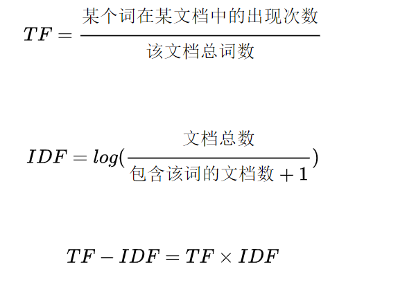
在所有文档中一个词的 IDF 是一样的TF 是不一样的。在一个文档中一个词的 TF 和 IDF
越高说明该词在该文档中出现得多在其他文档中出现得少。因此该词对这个文档的重要性较高可以用来区分这个文档。
import jieba
from sklearn.feature_extraction.text import TfidfVectorizer

def tokenizer_jieba(line):
    # 结巴分词
    return [li for li in jieba.cut(line) if li.strip() != '']

def tokenizer_space(line):
    # 按空格分词
    return [li for li in line.split() if li.strip() != '']

def get_data_tf_idf(email_file_name):
    # 邮件样本已经分好了词词之间用空格隔开所以 tokenizer=tokenizer_space
    vectoring = TfidfVectorizer(input='content', tokenizer=tokenizer_space, analyzer='word')
    content = open(email_file_name, 'r', encoding='utf8').readlines()
    x = vectoring.fit_transform(content)
    return x, vectoring
6 训练分类器
这里学长简单的给一个逻辑回归分类器的例子
from sklearn.linear_model import LogisticRegression
from sklearn import svm, ensemble, naive_bayes
from sklearn.model_selection import train_test_split
from sklearn import metrics
import numpy as np

if __name__ == "__main__":
    np.random.seed(1)
    email_file_name = 'all_email.txt'
    label_file_name = 'label.txt'
    x, vectoring = get_data_tf_idf(email_file_name)
    y = get_label_list(label_file_name)

    # print('x.shape : ', x.shape)
    # print('y.shape : ', y.shape)

    # 随机打乱所有样本
    index = np.arange(len(y))
    np.random.shuffle(index)
    x = x[index]
    y = y[index]

    # 划分训练集和测试集
    x_train, x_test, y_train, y_test = train_test_split(x, y, test_size=0.2)

    clf = svm.LinearSVC()
    # clf = LogisticRegression()
    # clf = ensemble.RandomForestClassifier()
    clf.fit(x_train, y_train)
    y_pred = clf.predict(x_test)
    print('classification_report\n', metrics.classification_report(y_test, y_pred, digits=4))
    print('Accuracy:', metrics.accuracy_score(y_test, y_pred))
7 综合测试结果
测试了2000条数据使用如下方法
-
支持向量机 SVM
-
随机数深林
-
逻辑回归
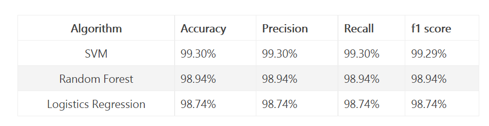
可以看到2000条数据训练结果200条测试结果精度还算高不过数据较少很难说明问题。
8 其他模型方法
还可以构建深度学习模型
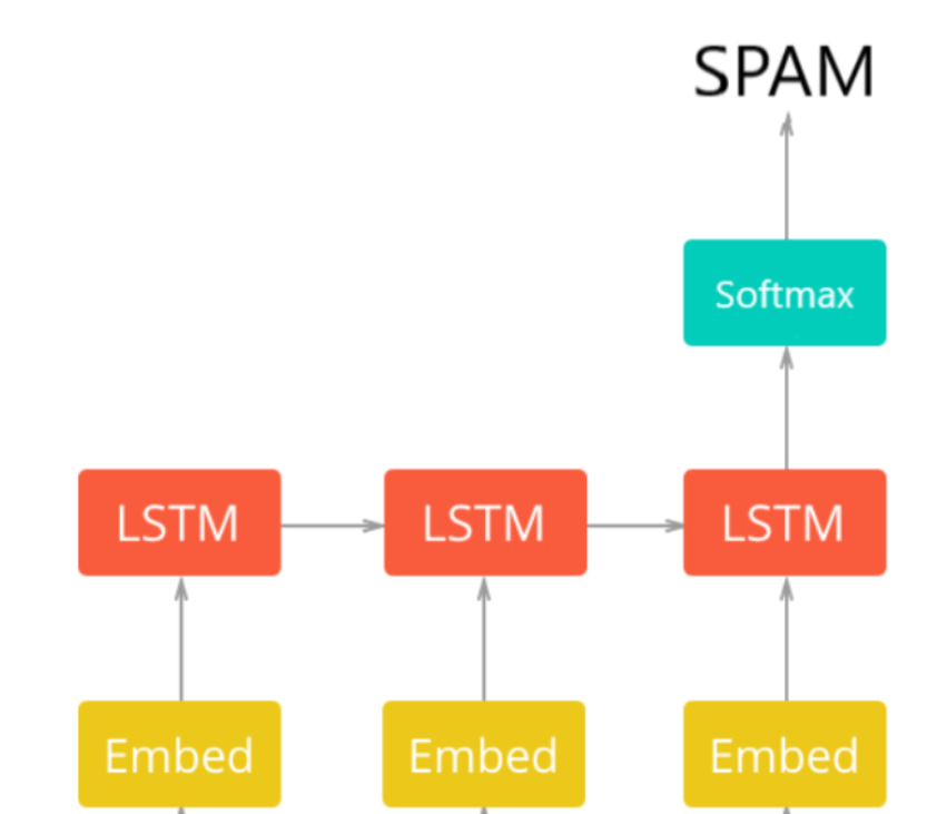
网络架构第一层是预训练的嵌入层它将每个单词映射到实数的N维向量EMBEDDING_SIZE对应于该向量的大小在这种情况下为100。具有相似含义的两个单词往往具有非常接近的向量。
第二层是带有LSTM单元的递归神经网络。最后输出层是2个神经元每个神经元对应于具有softmax激活功能的“垃圾邮件”或“正常邮件”。
    def get_embedding_vectors(tokenizer, dim=100):
    embedding_index = {}
    with open(f"data/glove.6B.{dim}d.txt", encoding='utf8') as f:
    for line in tqdm.tqdm(f, "Reading GloVe"):
    values = line.split()
    word = values[0]
    vectors = np.asarray(values[1:], dtype='float32')
    embedding_index[word] = vectors

    word_index = tokenizer.word_index
    embedding_matrix = np.zeros((len(word_index)+1, dim))
    for word, i in word_index.items():
    embedding_vector = embedding_index.get(word)
    if embedding_vector is not None:
    # words not found will be 0s
    embedding_matrix[i] = embedding_vector

    return embedding_matrix


    def get_model(tokenizer, lstm_units):
    """
    Constructs the model,
    Embedding vectors => LSTM => 2 output Fully-Connected neurons with softmax activation
    """
    # get the GloVe embedding vectors
    embedding_matrix = get_embedding_vectors(tokenizer)
    model = Sequential()
    model.add(Embedding(len(tokenizer.word_index)+1,
    EMBEDDING_SIZE,
    weights=[embedding_matrix],
    trainable=False,
    input_length=SEQUENCE_LENGTH))

    model.add(LSTM(lstm_units, recurrent_dropout=0.2))
    model.add(Dropout(0.3))
    model.add(Dense(2, activation="softmax"))
    # compile as rmsprop optimizer
    # aswell as with recall metric
    model.compile(optimizer="rmsprop", loss="categorical_crossentropy",
    metrics=["accuracy", keras_metrics.precision(), keras_metrics.recall()])
    model.summary()
    return model
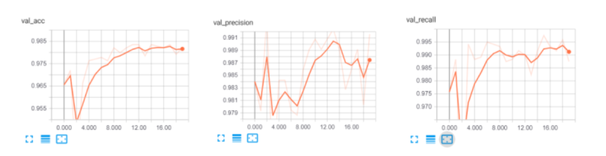
训练结果如下
_________________________________________________________________
Layer (type) Output Shape Param #
=================================================================
embedding_1 (Embedding) (None, 100, 100) 901300
_________________________________________________________________
lstm_1 (LSTM) (None, 128) 117248
_________________________________________________________________
dropout_1 (Dropout) (None, 128) 0
_________________________________________________________________
dense_1 (Dense) (None, 2) 258
=================================================================
Total params: 1,018,806
Trainable params: 117,506
Non-trainable params: 901,300
_________________________________________________________________
X_train.shape: (4180, 100)
X_test.shape: (1394, 100)
y_train.shape: (4180, 2)
y_test.shape: (1394, 2)
Train on 4180 samples, validate on 1394 samples
Epoch 1/20
4180/4180 [==============================] - 9s 2ms/step - loss: 0.1712 - acc: 0.9325 - precision: 0.9524 - recall: 0.9708 - val_loss: 0.1023 - val_acc: 0.9656 - val_precision: 0.9840 - val_recall: 0.9758

Epoch 00001: val_loss improved from inf to 0.10233, saving model to results/spam_classifier_0.10
Epoch 2/20
4180/4180 [==============================] - 8s 2ms/step - loss: 0.0976 - acc: 0.9675 - precision: 0.9765 - recall: 0.9862 - val_loss: 0.0809 - val_acc: 0.9720 - val_precision: 0.9793 - val_recall: 0.9883
9 最后
更多资料, 项目分享
https://gitee.com/dancheng-senior/postgraduate
| 阿里云国内75折 回扣 微信号:monov8 |
| 阿里云国际,腾讯云国际,低至75折。AWS 93折 免费开户实名账号 代冲值 优惠多多 微信号:monov8 飞机:@monov6 |